
Modeling Steps
The integration of USACE‑SWD algorithms in RiverWare brings together the RiverWare object-oriented modeling features, the power and flexibility of the priority rulebased simulation, and the Computational Subbasin, that allows the execution of multi-object computations from a rule function. The algorithms are thus implemented in modular, object-specific contexts for ease of maintenance and extension, as well as flexibility of use through user selectable methods. Following is a brief overview of the modeling steps and components.
Figure 1.1 shows the typical modeling steps to implement the functionality described in this document. An overview of each step is described in the following sections and the remainder of this document describes these items in detail.
Figure 1.1 Modeling steps diagram
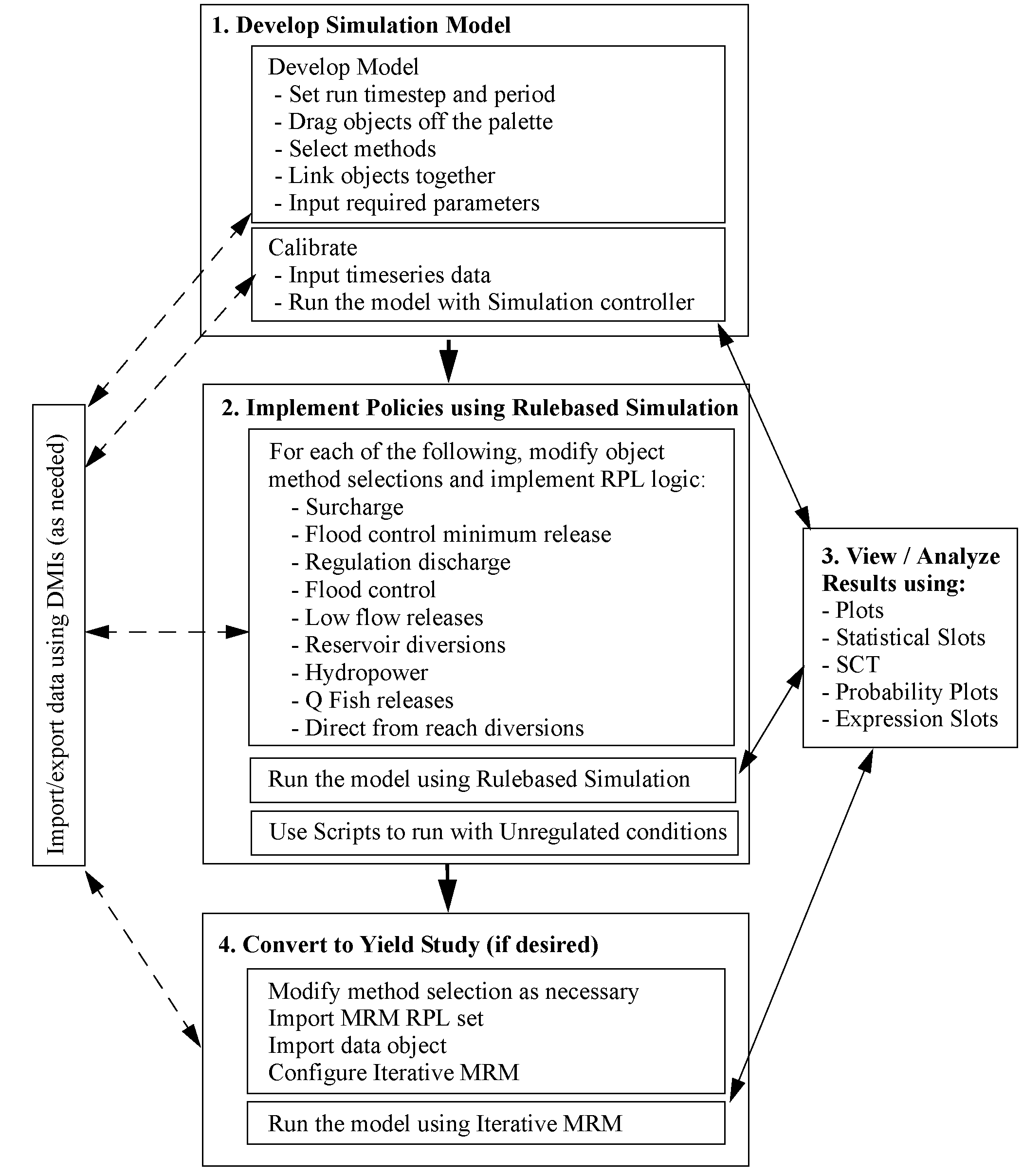
Develop Simulation Model
The first step is to develop a simulation model of the system by pulling objects off the palette, selecting the appropriate methods, linking objects together and specifying required data. Next, timeseries data is specified. The data management interface (DMI) can be used to import data as desired. With enough data, the model will run. At any point, the output utilities can be used to analyze and view results. The model should be calibrated to make sure that the inputs are producing the desired outputs. For example, you may input inflows to the system and reservoir outflows. You would then make sure that reservoir pool elevation or storage are correct and that downstream flows are routed correctly.
See Developing the Simulation Model for details.
Implement Policies Using Rulebased Simulation
The model can then be converted to a predictive mode by removing some of the inputs (E.g. Storage, Pool Elevation, and Outflows) to under-determine it. Then, rules can be implemented to compute the reservoir outflows based on the state of the system and the operating policies.
Described in this document are the following policies: surcharge, regulation discharge, flood control, low-flow releases, reservoir diversions, hydropower releases, and fish releases. Each policy may have additional methods to be selected and data to be input. Then, rules can be written in the RiverWare Policy Language (RPL). Many of the rules use specific predefined functions that execute methods on objects.
See Implementing Operating Policies Using Rulebased Simulation for details.
Run Using Unregulated Conditions
Sometimes, it is desired to run the model and compute the flows that would have occurred without one or more reservoirs in place. To do so, use scripts to change the model to use unregulated conditions. Use a script to make a run and generate snapshots of desired slots.
See Modeling Unregulated Conditions for details on defining and running an unregulated system.
View and Analyze Results
Given the model and the ruleset, a run is made. There are numerous tools and utilities that can be used to view and analyze results including the following:
• Plotting: present a graphical view of the data.
• Statistical slots: create frequency duration or exceedence curves. Then, plot them on a probability scale.
• Expression slots: create user defined expressions involving slot or other values. For example, this can be used for aggregation of data.
• Data Management Interface: DMIs can be used to export data to an external sink.
• System Control Table: SCTs can be used to view and edit data in a spreadsheet like format.
See Analysis and Output Tools for details on viewing and Analyzing results.
Convert to Yield Study, If Desired
A yield study is used to determine the largest constant diversion that can be made from a single reservoir such that the reservoir pool elevation will not drop down below the bottom of conservation pool at any time during the run period. Other operating policies like Surcharge, Regulation Discharge, Flood Control, Low-flow Release, and Hydropower are included in this analysis.
The Yield study uses the iterative Multiple Run Management configuration. In this configuration, the model is run multiple times with a different trial value for the diversion from a reservoir. After each run, logic is used to determine if the yield has been met and if not, a new trial value is calculated and a new run is made. Multiple reservoir can be included; each reservoir’s yield is computed separately, starting at the top of the system. Once the first reservoir’s yield is found, the next downstream reservoir’s yield is found. Thus, the model is run multiple times to find the yield from one reservoir, then that reservoir’s yield is locked in and the analysis is repeated on the next reservoir.
An existing model is converted to a yield study by importing data and an MRM RPL set. Then, the user sets up an MRM configuration and specifies the search algorithm (Bisection or a heuristic approach). The user can also specify the convergence criteria including the initial trial values and the maximum iterations. Finally, the run is made. The SCT can then be used to view the results of the multiple runs. Included in the results (for each reservoir) is the yield, the critical draw down date, the critical draw down period and the critical period duration.
The conversion to a yield study is a separate modeling step that may or may not be required for a given basin or portion of a basin. See Computing Reservoir Yield for complete details.
Revised: 08/04/2020