
Optimization Diagnostics
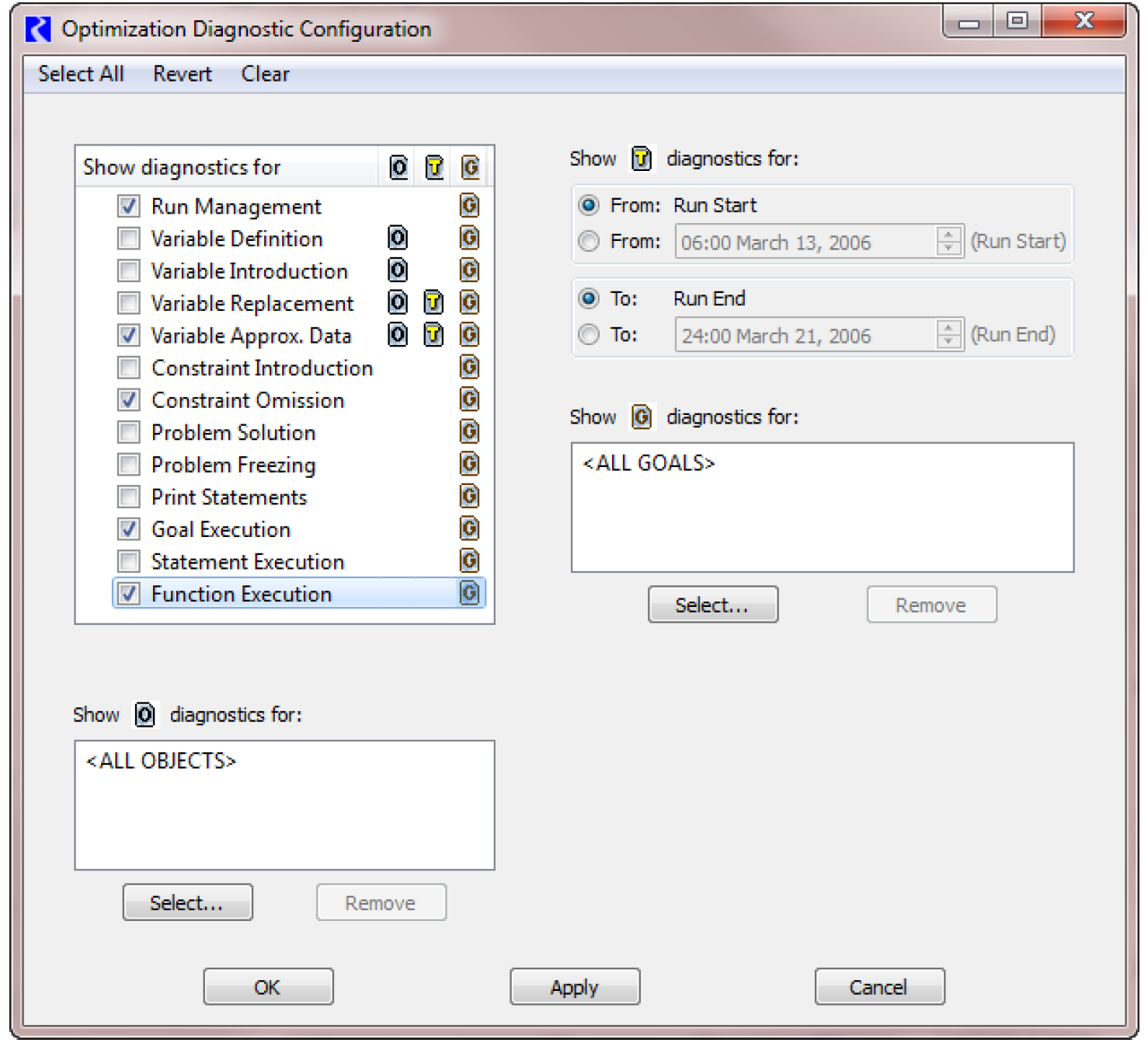
The Optimization Diagnostics Configuration dialog allows you to select from thirteen diagnostics groups and three context filters which are relevant during a Optimization run. This dialog’s settings are only valid when the Optimization controller is selected. It is accessed from the Optimization button on the Diagnostics Manager.
Figure 3.13
Optimization Diagnostic Groups
Table 3.4 summarizes the types of messages that are displayed when a Diagnostic Group is selected.
Diagnostics Group | Type of diagnostics issued |
|---|---|
Run Management | Beginning/End of Run and each goal. Examples: • Initializing model run. • Beginning of run. • Begin goal. • Execute goal. • End goal • End of run. |
Variable Definition | Diagnostic messages for definition of each variable: • Defining the variables of slot "SM3 reservoir.Pool Elevation" in terms of variables on the shifted slot "Shifted Pool Elevation" (shift = -320.00000000 "m^1"). • Adding definition "Shift Scaling of Pool Elevation" for the following variables: SM3 reservoir.Pool Elevation [t] • ... Definition: ( SM3 reservoir.Pool Elevation [t] == ( SM3 reservoir.Shifted Pool Elevation [t] - -320.00000000 "m^1" ) ) |
Variable Introduction | Diagnostic messages for introduction of new decision variables: • While preparing for the run, encountered the new decision variable "SM3 reservoir.Outflow [24:00 October 31, 2117]"; to define this variable 1 constraints will be introduced into the optimization problem. • While executing statement 3.1.1(date=24:00 October 31, 2092).1, encountered the new decision variable "SM3 reservoir.Opt piece for Power.4 [24:00 October 31, 2092]"; to define this variable 1 constraints will be introduced into the optimization problem. |
Variable Replacement | Diagnostic messages for replacement of variables: • While executing statement 1.1.1(date=24:00 March 31, 2100).1, replacing one constraint with another. • ... Constraint being replaced: ( ( 1.00000000 * SM3 reservoir.Shifted Pool Elevation [24:00 March 31, 2100] ) <= 87.00000000 "m^1" ) • ... Replacement constraint: ( SM3 reservoir.Storage [24:00 March 31, 2100] <= 12642800000.00000000 "m^3" ) |
Variable Approx. Data | Diagnostic messages for approximation of data: • The constraint "( ( 1.00000000 * Wilbur.Bypass Capacity [18:00 March 13, 2006] ) >= 1.13267386 "m^3 / s^1" )" was determined to be ineffective while attempting to substitute an equivalent constraint on "Wilbur.Storage" using the table "Wilbur.Bypass Capacity Table". The constraint has been ignored because it is redundant for all values in the table, which may need additional values. The nearest value in the table is 1.982179 cms. If this constraint was indirectly generated by RiverWare, prior diagnostic messages or turning on informational diagnostics may be helpful. This warning is issued for this constraint once per run, although this situation might hold for multiple dates. The data table is automatically generated at the beginning of each run based on "Wilbur.Bypass Table", so data corrections should be made there. |
Constraint Introduction | Diagnostic messages for introduction and linearization of constraints: • Adding the defining constraint "(Def.) Economic Value.Linear Avoided Operating Cost [24:00 September 30, 2085], Linear Avoided Operating Cost Replacement" to the optimization problem. • ... Original constraint: ( SM3 reservoir.Power [24:00 June 30, 2110] >= 100.00000000 "MW" ) • ... Linearized constraint: ( ( ( ( ( ( ( ( 3.00965758 "1000000.000000 kg^1 / m^1-s^2" * SM3 reservoir.Opt piece for Power [24:00 June 30, 2110] ) + ( 2.98868019 "1000000.000000 kg^1 / m^1-s^2" * SM3 reservoir.Opt piece for Power.1 [24:00 June 30, 2110] ) ) + ( 2.97411902 "1000000.000000 kg^1 / m^1-s^2" * SM3 reservoir.Opt piece for Power.2 [24:00 June 30, 2110] ) ) + ( 2.95792886 "1000000.000000 kg^1 / m^1-s^2" * SM3 reservoir.Opt piece for Power.3 [24:00 June 30, 2110] ) ) + ( 2.90415559 "1000000.000000 kg^1 / m^1-s^2" * SM3 reservoir.Opt piece for Power.4 [24:00 June 30, 2110] ) ) + ( 2.77190824 "1000000.000000 kg^1 / m^1-s^2" * SM3 reservoir.Opt piece for Power.5 [24:00 June 30, 2110] ) ) + ( 2.20884309 "1000000.000000 kg^1 / m^1-s^2" * SM3 reservoir.Opt piece for Power.6 [24:00 June 30, 2110] ) ) >= 100.00000000 "1000000.000000 m^2-kg^1 / s^3" ) |
Constraint Omission | Diagnostic messages when constrains are skipped as they will have no effect. • Attempt to add a soft constraint "C22.1.1(res=Wilson).1(date=12:00 March 21, 2006).1 70" which would not constrain the problem (e.g., it might be weaker than the restrictions imposed by the bounds on the variables), so it is not being added. The full constraint is: ( ( 1.00000000 * Wilson.Outflow [12:00 March 21, 2006] ) >= 0.14158423 "1000.000000 m^3 / s^1" ) • Skipping the new constraint C25.1.1(res=Apalachia).1(date=24:00 March 21, 2006).1 36 because the left-hand side is already bounded by other constraints (C11.1.1(res=Apalachia).1(date=24:00 March 21, 2006).1 1 A and C11.1.1(res=Apalachia).1(date=24:00 March 21, 2006).1 1 B). Currently, 67204983.66069999 "m^3" <= lefthand side <= 67204983.66069999 "m^3". |
Problem Solution | Diagnostic messages for solving the optimization problem and the number of variables and constraints that are freezing • Freezing 0 variables. • Freezing 0 constraints. • While executing statement 2.1, defining a REPEATED MAXIMIN objective involving 2 constraints and solving the problem. • ... Objective: ( 100.00000000 * ZM2.1 ) • ... Original objective: (... • ... Linearized objective (... |
Problem Freezing | Diagnostic messages for freezing variables and constraints • Frozen constraint: Ending Pool Elevation, C2.1.1(date=24:00 September 30, 2119).1 1 B: was 267.970000 <= ... <= 267.970000 (dual cost = 30.567953). Current statement: CONSTRAINT $ "SM3 reservoir.Pool Elevation" [date] == $ "Opt Data.Ending Elevation" [date] • Frozen variable: ZM3.1 = 0.100000 (reduced cost = 100.000000) |
Print Statements | User defined messages within rules for each goal. Example: • Minimum Load goal was successful. |
Goal Execution | Diagnostic messages displaying when a goal is executed: • Executing goal #3 ("MinimumLoad", within group "Firm Energy") |
Statement Execution | Diagnostic messages displaying when each statement within a goal is executed • Executing CONSTRAINT statement 3.1.1(date=24:00 September 30, 2119).1, which will attempt to add the soft constraint: ( SM3 reservoir.Power [24:00 September 30, 2119] >= 100.00000000 "MW" ). • Executing REPEATED MAXIMIN statement 1.1. |
Function Execution | Diagnostics messages for function execution (both user defined and predefined). “Before Execution” function diagnostics show the function being called and the arguments passed into the function. “After Execution” function diagnostics show the value that the function evaluated to and whether or not the value was constrained. Note: Function diagnostics also need to be enabled on the functions themselves. This can be done through the Function Editor dialog (for enabling diagnostics on individual functions) or by selecting Ruleset, then Ruleset Function Diagnostics from the main RPL Set Editor (for enabling or disabling function diagnostics for all functions in the ruleset). See Function Diagnostics for details. • GetMaxReleaseGivenInflow (% “WattsBar”, 0.634 [“1000 * cms”], @”Start Timestep”) • “GetMaxReleaseGivenInflow” evaluated to: 1299.413 [“cms”] |
Init. Rules Rule Execution | Initialization Rules rule execution diagnostics are printed for each rule. For an Optimization run, there is no filtering based on rule name. When enabled, diagnostics are shown for all Initialization rules. Examples: • Executing rule (#3) Assignment initiated (the left-hand side is “Mohave.Storage”[]) Evaluation of Assignment statement successful; will attempt assignment Mohave.Storage[July, 1998] = 1590800.00 [1.00 acre-ft] Rule successfully finished • Early termination: NaN encountered. The problem was encountered at the following location within the expression: “FC Violation”(). • RHS of assignment evaluated to NaN. |
Init. Rules Function Execution | Diagnostics messages for function execution (both user defined and predefined) from initialization rules. For an Optimization run, there is no filtering based on rule name. When enabled, diagnostics are shown for all Initialization rules. “Before Execution” function diagnostics show the function being called and the arguments passed into the function. “After Execution” function diagnostics show the value that the function evaluated to and whether or not the value was constrained. Note: Function diagnostics also need to be enabled on the functions themselves. This can be done through the Function Editor dialog (for enabling diagnostics on individual functions) or by selecting Ruleset, then Ruleset Function Diagnostics from the main Ruleset Editor (for enabling or disabling function diagnostics for all functions in the ruleset). See Function Diagnostics for details. Examples: • GetMaxReleaseGivenInflow (% “WattsBar”, 0.634 [“1000 * cms”], @”Current Timestep”) • “GetMaxReleaseGivenInflow” evaluated to: 1299.413 [“cms”] • “GetMaxReleaseGivenInflow” constrained to: 1200.00 [“cms”] |
Init. Rules Print Statements | User defined messages for each initialization rule. For an Optimization run, there is no filtering based on rule name. When enabled, diagnostics are shown for all Initialization rules. Example: • Entering rule curve routine for January - July |
Revised: 08/02/2021