
RPL Optimization Goal Set
The operating policy of a basin is expressed in a RPL Optimization Goal Set. This section describes the components of the Optimization Goal Set. An Optimization Goal Set uses much of the same syntax as a Rulebased Simulation ruleset. See Managing RPL Sets in RiverWare Policy Language (RPL) for details.
Key differences between the formulation of rules and Optimization goals are described in the following sections.
Prioritized Policy
In Optimization, each aspect of the basin operating policy is expressed in a goal, and each goal is given a unique priority. In this way, goals for Optimization are analogous to rules for Rulebased Simulation. The contents of each goal are either constraints or objectives. See Goal Types and Statements in Goal Sets for details about the contents of goals. This section focuses on the top level structure of the goal set.
RBS rules execute from lowest priority to highest priority. Optimization goals on the other hand, execute from highest priority to lowest priority (lowest number to highest number). Each priority that contains an objective, either a Maximize or Minimize objective or a Soft Constraint Set derived objective, will trigger a solution of the Optimization problem. The problem at each priority will include the constraints from all higher priority goals, along with their maximized satisfaction, and any new constraints added at the current priority. Thus at each priority, degrees of freedom are removed from the problem reducing the solution space. If the goal contains only hard constraints, or if the logic in the goal results in no new constraints getting added to the Optimization problem, then there will not be a new solution of the Optimization problem at that priority.
RBS rules are normally ordered to execute in an upstream to downstream order, object-by-object. Generally there is no need to order Optimization goals in an upstream to downstream order. The priorities of the goals should correspond to their true priorities in operations. The highest priority goals should correspond to the most important operating constraints, those that should essentially never be violated.
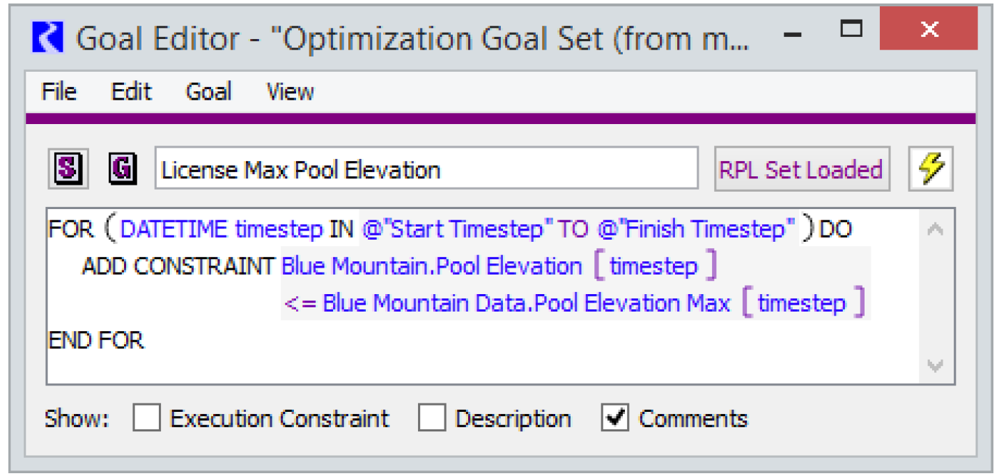
A single goal can contain constraints for multiple objects, but it is generally recommended that a single goal correspond to a single operating policy. For example, the highest priority goal might contain the license maximum Pool Elevation constraints for all reservoirs at all timesteps. The second goal might contain the license minimum Pool Elevation constraints for all reservoirs at all timesteps. This is generally better practice than placing the minimum and maximum elevation constraints in the same goal or placing the minimum elevation constraint in the same goal (same priority) as a minimum flow constraint. When multiple policies are combined in a single goal, it is not always obvious how the policies will trade off with one another if it is not possible to satisfy all constraints at that priority.
Medium priority goals generally contain constraints that you expect to get satisfied most of the time but that may not be possible to satisfy under some operating conditions, for example under extreme high or low flows. Lower priority goals typically contain target operating constraints, targets that you would like to meet under ideal conditions but are expected to be frequently violated due to higher priority constraints and input data (e.g. inflows). For example, you might have a low priority goal to keep flows equal across all reservoirs on each timestep, but most of the time you cannot keep flows exactly equal due to other requirements on the system. Typically the lowest priority contains an objective function to optimize with the remaining degrees of freedom given all higher priority constraints. For example, the objective might maximize the total value of hydropower generation during the run within the operational limits specified by higher priority constraints.
Figure 4.1 is a simple example of an Optimization Goal Set.
Figure 4.1
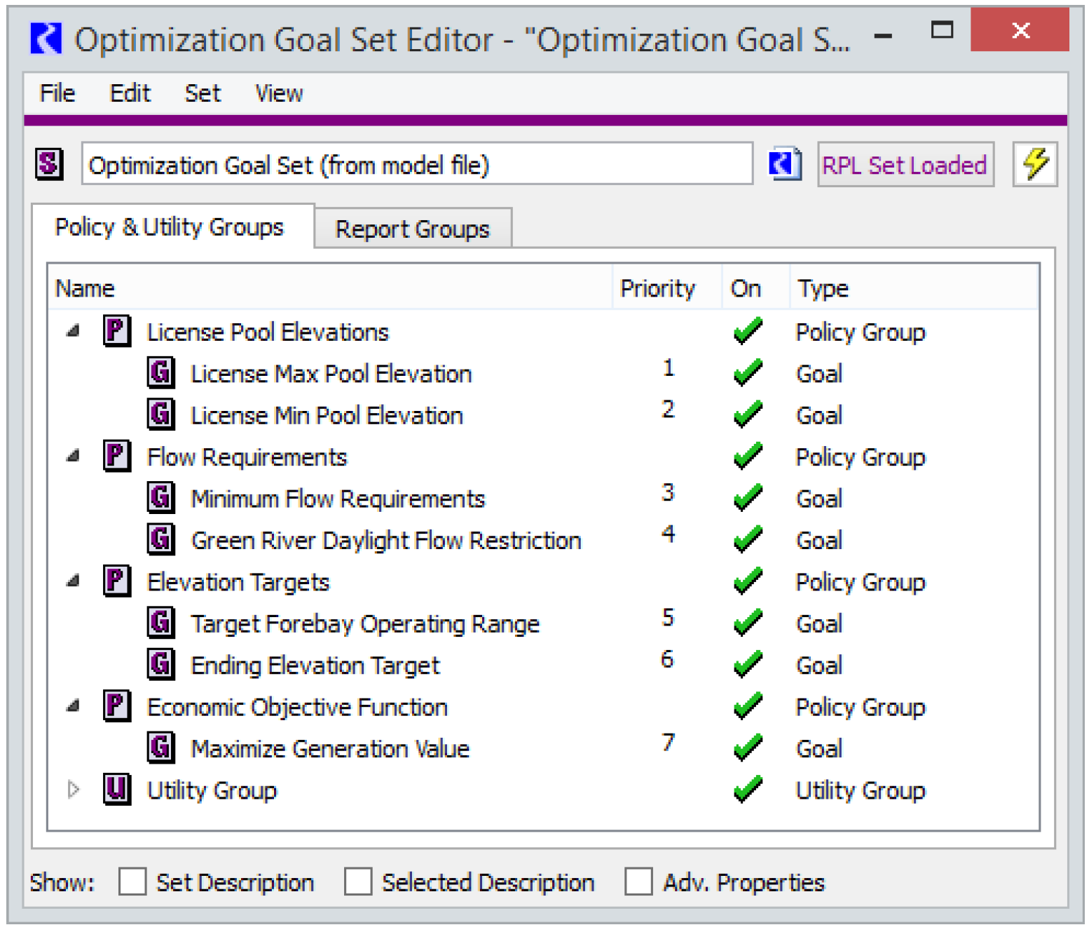
In this goal set, the License Max and Min Pool Elevations are at the highest priorities. You would therefore expect that these elevation limits are almost never violated. The Minimum Flow Requirement is at the next priority, so you would also expect it to be satisfied most of the time. However, if there were a case with low flows and it was not possible to meet both the minimum elevation requirement and the minimum flow requirement, then the solution would meet the minimum elevation and would violate the minimum flow requirement. It would get the flow as close to the minimum as possible, and in doing so, it would take the reservoirs to the minimum elevation.
The Target Forebay Operating Range goal is at a lower priority. This suggests that ideally you would like to keep the forebays (Pool Elevation) within some specified range, but you are not going to violate either of the flow requirements in goals 3 and 4 to do so.
The final goal is maximizing the value of generation. Normally an objective such as this would use as much water as possible to produce as much generation as possible. The Ending Elevation Target goal at priority 6 is likely in place to prevent the maximum value goal from draining all reservoirs to the bottom of their operating range. The solution will only maximize the economic value of generation within the limits specified by the higher priority goals. It can only use the degrees of freedom that remain after solving to meet all of the higher priority constraints. The solution would go outside of the target forebay operating range (priority 5) if necessary to meet a flow requirement (priority 3 or 4), but it would not go outside of the target operating range just to increase the generation value (priority 7).
Note: In practice, most Optimization Goal Sets contain many more goals than the example shown here in order to model all of the operational requirements the system.
Note: All the goals correspond to operational policies. There are no goals added to express the physical constraints that define the system (e.g. mass balance and routing). All physical constraints get included in the Optimization problem automatically by RiverWare (see Physical Constraints). There is no need for the user to formulate the physical constraints.
Like rulesets, Optimization Goal Sets can be organized into policy groups and utility groups, as seen in the example above. The policy groups contain goals and the utility groups contain functions used within the goals. As with rules, the policy groups are for organizational purposes only. The solution evaluates each goal individually in priority order. It does not solve by policy group. Priorities of individual goals and policy groups can be shifted by clicking and dragging the goal/group name to the new priority location. Individual goals and policy groups can be activated and deactivated by clicking on the green check mark or red  next to the goal or policy group name.
next to the goal or policy group name. 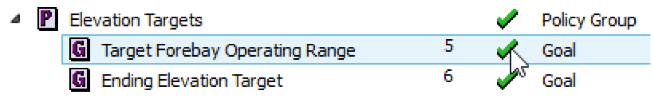
Clicking on the green check mark will change it to a red  .
.
.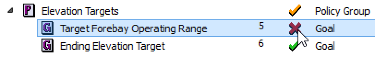
Clicking on the red  will reactivate the goal or policy group and change it back to a green check mark.
will reactivate the goal or policy group and change it back to a green check mark.Goal Types
Technically there is only a single type of goal that is added to a goal set. However, goals can be thought of as falling in one of three general categories: hard constraints, soft constraints, and objectives. Like rules, Optimization goals consist of statements. The goal type is determined by the type of statements that are added to it. See Statements in Goal Sets for descriptions of the types of statements that can be added to a goal. The goal types are described in the following sections.
Hard Constraints
A hard constraint goal includes Constraint statements (see Constraint) that are not within a Soft Constraint Set derived objective (see Soft Constraint Set). A goal with only hard constraints does not trigger a solution of the Optimization problem. It only adds new constraints to the problem. The constraints will not have an effect on the solution until the next priority that includes either a Soft Constraint Set derived objective or a Maximize or Minimize objective.
Hard constraints should be used with caution. If any hard constraint cannot be fully satisfied at the next priority with a solution, then an infeasible solution (i.e. no solution) will be returned. These infeasibilities can often be difficult to debug. It can be tempting to consider the highest priority operating constraints as hard constraints that are never violated, for example, a license Pool Elevation limit. However it is better practice to formulate these highest priority policies as soft constraints at the highest priorities in the goal set. Once the soft constraints are satisfied at a high priority, they will effectively be treated as hard constraints when solving at all remaining priorities. In the rare case that the high priority constraints cannot be fully satisfied, the soft constraint approach will still return a solution rather than an infeasibility. The solution returned will provide the user with more information about where, when and why the violation occurred than if the model simply returns an infeasible solution.
Figure 4.2 is an example of a technically valid hard-constraint formulation.
Figure 4.2
However, it is recommended instead that the contents of goal such as this with operational policy be placed within a Soft Constraint Set derived objective statement.
One common use of hard constraints is to formulate the defining constraints for user-defined variables (see User-defined Variables). In fact, defining constraints are typically the only recommended use of hard constraints. Again, these defining, hard constraints should be formulated in a manner that they are guaranteed to always be feasible. They are typically placed at the highest priorities in the goal set.
Soft Constraints
The large majority of goals in an Optimization Goal Set are typically soft constraint goals. These goals have a Soft Constraint Set derived objective statement (see Soft Constraint Set) at the top level within the goal, and within the Soft Constraint Set statement are one or more Constraint statements. The Soft Constraint Set triggers a solution of the optimization problem as long as the goal actually adds new constraints to the problem. (Some goals may contain logic to only add constraints under certain conditions, for example seasonal constraints. If the logic within the goal results in no new constraints being added, then there is no need for a solution after the goal is processed because there is no change to the Optimization problem.) RiverWare automatically converts the goal into a derived objective to maximize the satisfaction of the constraints in the goal given the objective value (satisfaction level) of all higher priority goals. RiverWare provides four different approaches for maximizing the satisfaction of soft constraints (see Derived Objectives). See Soft Constraint Set for details on implementing soft constraints.
Soft constraint goals should be used to formulate all operational constraints (e.g. Pool Elevation limits, minimum Outflow requirements, minimum Power generation requirements, etc.). They are also often used for lower priority target operations and solution quality constraints, constraints that prevent the Optimization solution from exploiting remaining degrees of freedom to produce operations that would never be carried out in practice. These lower priority target constraints are usually not expected to be satisfied under all conditions.
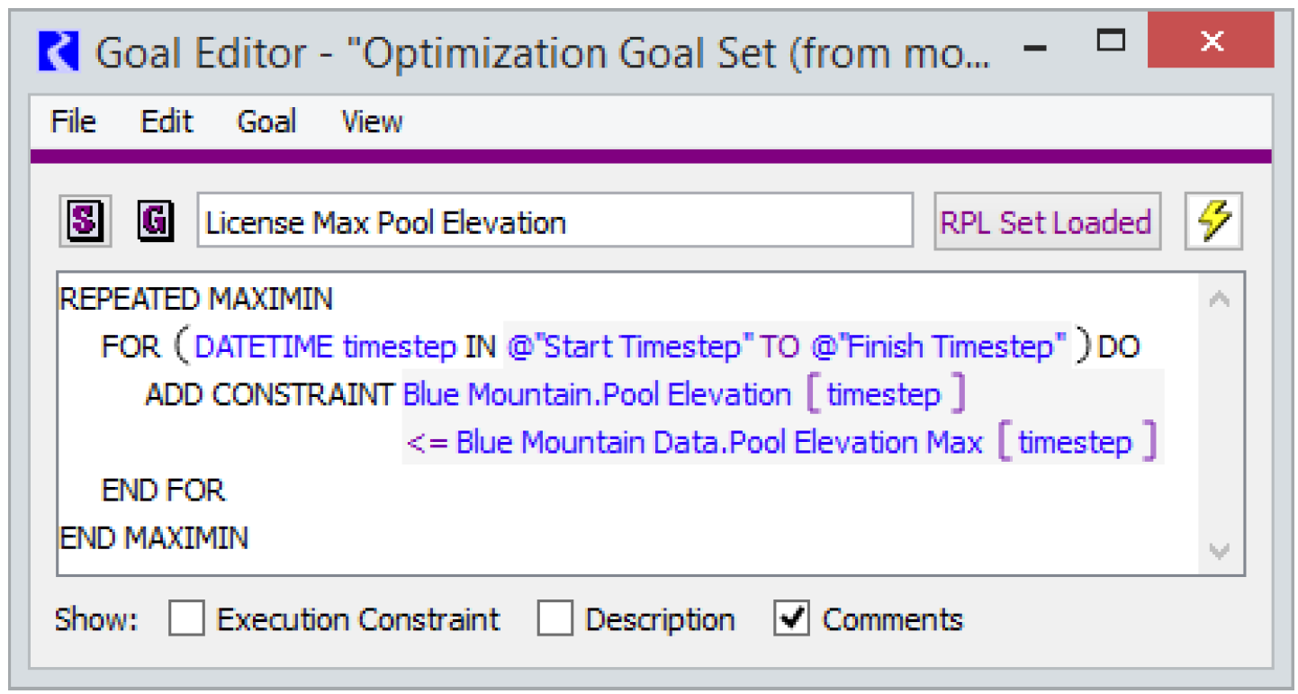
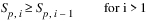
Figure 4.3 is an example of a maximum Pool Elevation policy formulated as a soft constraint goal using the Repeated Maximin derived objective.
Figure 4.3
Objectives
Objective goals are used to maximize or minimize a specified quantity. Technically, and objective maximizes a linear expression of variables. For example, the objective might maximize the total value of hydropower generation over the entire run period.
Typically objectives are at or near the lowest priorities in the goal set. They maximize/minimize the objective given any remaining degrees of freedom after all higher priority constraints. The solution from an objective goal will often use up most remaining degrees of freedom in the Optimization problem. See Objective for details on implementing an objective.
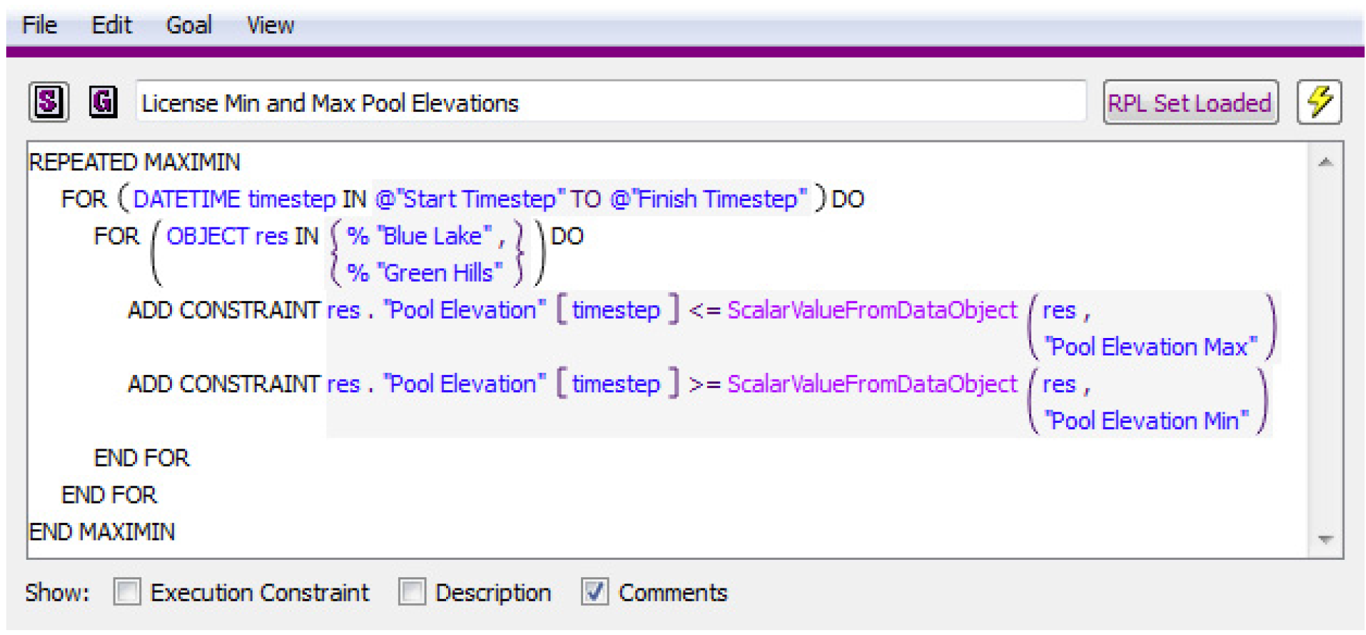
Figure 4.4 is an example of an objective to maximize the total system hydropower generation over the entire run.
Figure 4.4
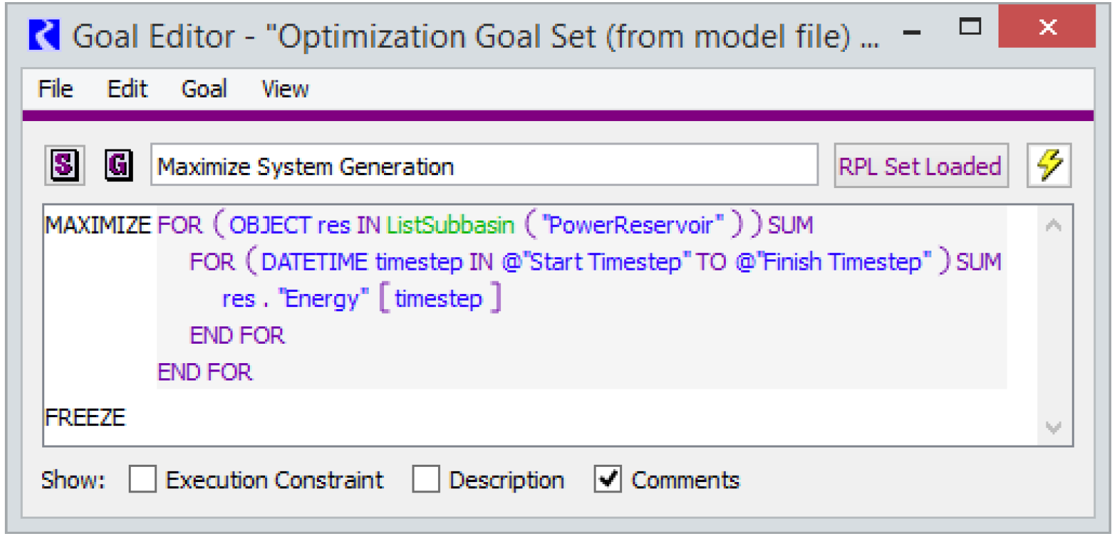
This goal loops over all power reservoirs in the model and over all timesteps and creates an expression that is the sum of the Energy variable (slot) for those reservoirs and timesteps. The objective maximizes that sum.
Statements in Goal Sets
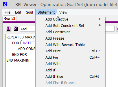
This section describes the pieces of an Optimization Goal. At the top level, an Optimization Goal consists of statements, which are available from the Statement menu in the RPL Viewer or Goal Editor dialog (see Figure 4.5). The list of available statements is slightly different than the list available for rules (see RPL Statements in RiverWare Policy Language (RPL)). A description of each is given below.
Figure 4.5
Objective
An Objective statement can be a minimize or maximize objective and has the form:
MAXIMIZE <expr>
or
MINIMIZE <expr>
The user then defines the expression to minimize or maximize. The expression within the objective statement may contain multiple terms and summations over multiple slots and/or timesteps as long as it is a linear combination of variables.
Note: A Freeze statement must be added at the end of an Objective statement in order to freeze the objective value. Otherwise the objective value from the goal will not necessarily be maintained at lower priorities.
Figure 4.6 is an example of an objective to maximize the total system hydropower generation over the entire run.
Figure 4.6

This goal loops over all power reservoirs in the model and over all timesteps and creates an expression that is the sum of the Energy variable (slot) for those reservoirs and timesteps. The objective maximizes that sum.
Soft Constraint Set
When a Soft Constraint Set is added, the Optimization solution will attempt to satisfy all of the constraints in the set completely. If it is not possible to fully satisfy all constraints introduced at the current priority due to physical conditions and/or higher priority goals, the solution will attempt to satisfy the constraints as fully as possible based on the one of the three available solution methods (derived objectives) described below. The satisfaction level of the constraint set is frozen once the Optimization problem has been solved at that priority (that is, once a constraint has been satisfied at a high priority, it will not be violated to meet a lower priority goal or objective).
Note: Only one Soft Constraint Set can be added to a goal, but a single Soft Constraint Set can contain multiple individual Constraint statements.
See Satisfaction Variables in Soft Constraints for the mathematical details about how constraint satisfaction is defined.
When you add a Soft Constraint Set, you select one of the following solution approaches to maximize satisfaction.
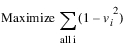
Summation
This approach will minimize the total deviation from the constraint values within the Soft Constraint Set (formally it maximizes the total satisfaction).
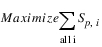
where there is one satisfaction variable Sp,i for each constraint i added at the current priority p.
The potential downside of this approach is that it can tend to place all of the deviation on one or just a few variables. For example, if a minimum flow constraint cannot be met for every timestep, it might minimize the total violation by satisfying the constraint at all but one timestep and putting a very large violation on that one timestep. Typically, this is not the preferred solution in a water resources context. The concentration of large violations when using a Summation Soft Constraint Set can be prevented by applying a With Reward Table statement within the Summation. See With Reward Table for details about using the With Reward Table statement. See Summation for details about the Summation derived objective.
Note: A Freeze statement must be added at the end of a Summation derived objective statement in order to freeze the objective value (satisfaction). Otherwise the satisfaction of the soft constraints from the Summation goal will not necessarily be maintained at lower priorities.
Single Maximin
Instead of minimizing the total violation, this approach will minimize the single largest violation (formally it maximizes the minimum satisfaction). This prevents a single, very large violation by spreading the violation out over multiple variables or timesteps.

where Sp is a single satisfaction variable applied to all constraints added at the current priority p.
The potential downside of this approach is that it does nothing to improve the satisfaction of the remaining constraints that are not contributing to the largest violation. This issue is addressed by the next type of derived objective, Repeated Maximin. See Single Maximin for details about the Single Maximin derived objective.
Note: A Freeze statement must be added at the end of a Single Maximin derived objective statement in order to freeze the objective value (satisfaction). Otherwise the satisfaction of the soft constraints from the Single Maximin goal will not necessarily be maintained at lower priorities.
Repeated Maximin
This approach begins with the single maximin. It then freezes the satisfaction of the largest violation and re-solves the problem by minimizing the next largest violation. It repeats this process until either all violations have been minimized or all remaining constraints are fully satisfied.
While Sp,i-1 < 1

where Sp,i is a single satisfaction variable applied to all constraints added at the current priority p that have not yet been frozen prior to the ith Repeated Maximin iteration.
The Repeated Maximin approach tends to spread out deviations as evenly as possible, which is often the desired solution in a water resources context. The potential downside of the Repeated Maximin approach is that in some cases it can require numerous iterations when it is not possible to satisfy all constraints. Depending on the size of the model this can cause a significant increase run time. The Summation approach always requires only a single solution at the given priority, so it tends to be faster, but it does not, in general, provide the same solution quality as Repeated Maximin. In some cases, a reasonable balance between solution quality and run time can be provided by applying a With Reward Table statement within a Summation. See With Reward Table for details about the Summation With Reward Table. See Repeated Maximin for details about the Repeated Maximin derived objective.
Constraint
Constraints are formulated as either <=, >= or == expressions. Constraint statements can be added within a Soft Constraint Set, a For statement, an If statement or a With statement (or within a nested combination of these statement types). If a Constraint statement is added that is not within a Soft Constraint Set, it will be treated as a hard constraint.
Note: It is not necessary to add physical constraints in Optimization Goals. Physical constraints are added automatically by RiverWare as needed based on the model topology and user-selected methods; see Physical Constraints for details.
The logical operators are added from the RPL Palette. The user can formulate a constraint with variables and/or scalar values on either side of the logical operator as long as all expressions within the constraint are linear combinations of variables and maintain dimensional consistency. RiverWare will automatically convert all constraints to a canonical form with variables (and coefficients, where applicable) on the left-hand-side and scalar values on the right-hand side when the Optimization problem is processed internally.
Figure 4.7 shows a goal containing basic minimum and maximum Pool Elevation constraints that are being added as Repeated Maximin soft constraints for two reservoirs for all timesteps in the run.
Figure 4.7
The minimum and maximum Pool Elevation values are being retrieved from slots on a data object corresponding to each reservoir by a user-defined function called ScalarValueFromDataObject.
Note: If and With expressions cannot be added within a Constraint statement. Also RPL predefined functions cannot be used within Constraint statements; however user-defined functions can be used within a Constraint statement as long as they result in linear constraint expressions. RPL predefined functions can be used in the outer level Optimization Goal statements that contain Constraint expressions, for example within the boolean expression of an If statement that contains a Constraint statement.
Freeze
A Freeze statement locks in the value of an objective after solving a minimize or maximize objective. A Freeze statement should be added after an objective statement when it is desired to actually preserve the solution resulting from solving the objective function (i.e. for standard optimization objectives). In some cases it might be necessary to maximize or minimize an objective to calculate values for ‘temporary’ use in the solution before solving the ‘true’ objective at a later priority. In this case, it is not desired to freeze value of the objective function for the final solution, and a Freeze statement would not be added.
Figure 4.8 shows a Freeze statement added after a typical objective to maximize the value of hydropower over the entire run. Freeze statements must also be added after Summation and Single Maximin Soft Constraint sets in order to lock in the derived objective value (preserve the constraint satisfaction). It is not necessary to add a Freeze statement after a Repeated Maximin Soft Constraint Set. The satisfaction variables for Repeated Maximin are frozen automatically.
Figure 4.8
With Reward Table
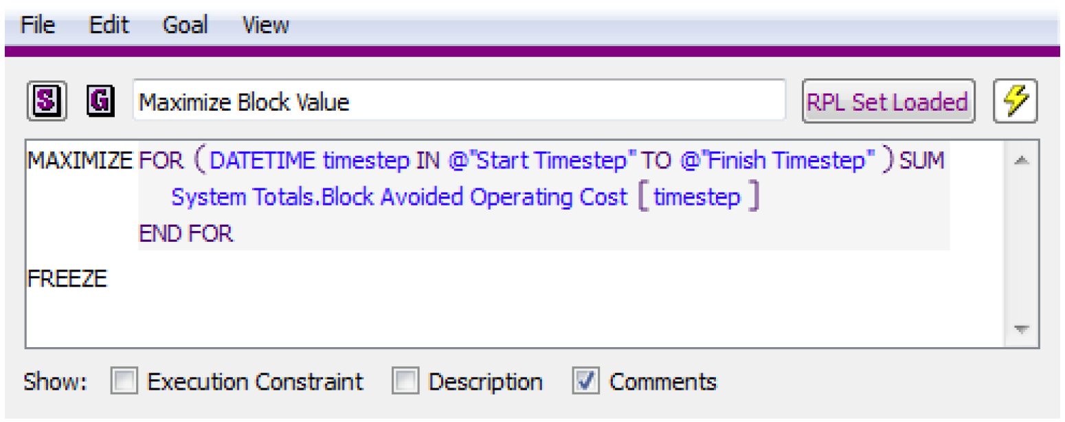
A With Reward Table statement allows a reward function to be applied to the satisfaction variables within a Summation objective for a soft constraint set. The With Reward Table statement can only be used within a Summation soft constraint set. Using the With Reward Table statement in any other context will result in an error. See Figure 4.9 for an example.
Figure 4.9
The reward table allows a piecewise function to be applied to the satisfaction variables within Summation objective. Instead of using the standard Summation derived objective for maximizing satisfaction, the derived objective becomes as follows:

where R is the reward function for the satisfaction variables.

Typically this approach is used to penalize larger violations more than smaller violations. For example, a common approach is to minimize the sum of squared violations. This tends to smooth out large violations by spreading them out over multiple time steps rather than concentrating large violations on a few time steps. Applying the appropriate reward function within a Summation soft constraint set can often produce a result that compares to the Repeated Maximin solution in terms of solution quality but has the benefit of only requiring a single solution at the given priority and can therefore be much faster.
The piecewise reward function must be described in a user created table slot. The table slot is given as an argument to the With Reward Table statement.
WITH REWARD TABLE <slot expr>
The reward table slot must have two columns with units of NONE. The first column contains satisfaction values. The second column contains the corresponding reward values. The values in both columns must be between 0 and 1. If the user does not include rows for a satisfaction of 0 and 1, RiverWare will add these rows internally when processing the piecewise reward function with values of 0 and 1 used for the reward. The reward table must be concave. (Reward must be a concave function of Satisfaction.)
An example is provided below for a reward table that corresponds to minimizing the sum of squared violations
Example 4.1 Example Reward Table: Minimize the Sum of Squared Violations
Conceptually the desired derived objective is to minimize the sum of squared violations.

Violations are scaled from 0 to 1, where 1 corresponds to the maximum violation based on a higher priority constraint or bound. Thus an equivalent objective to minimize the sum of squared violations is
For performance reasons, the RiverWare Optimization solution maximizes satisfaction variables rather than minimizing violations. See Soft Constraint Set for details about how the satisfaction variables are defined.

The maximize objective then becomes
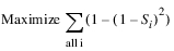
Table 4.1 shows how this can be described by a piecewise linear function that linearizes the function in 10 discrete segments.
vi | vi2 | si | 1 - vi2 |
|---|---|---|---|
1.0 | 1.00 | 0.0 | 0.00 |
0.9 | 0.81 | 0.1 | 0.19 |
0.8 | 0.64 | 0.2 | 0.36 |
0.7 | 0.49 | 0.3 | 0.51 |
0.6 | 0.36 | 0.4 | 0.64 |
0.5 | 0.25 | 0.5 | 0.75 |
0.4 | 0.16 | 0.6 | 0.84 |
0.3 | 0.09 | 0.7 | 0.91 |
0.2 | 0.04 | 0.8 | 0.96 |
0.1 | 0.01 | 0.9 | 0.99 |
0.0 | 0.00 | 1.0 | 1.00 |
The table entered in RiverWare is taken from the last two columns. See Figure 4.10 and Figure 4.11 for examples.
Figure 4.10
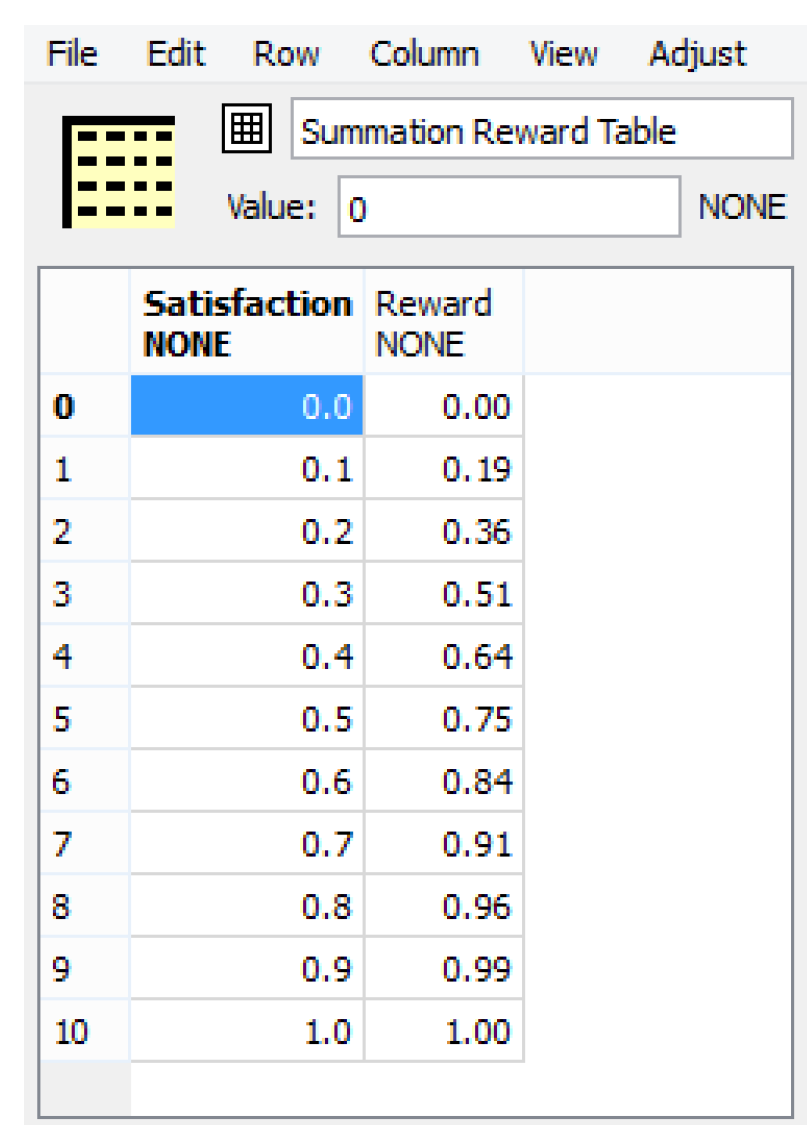
Figure 4.11
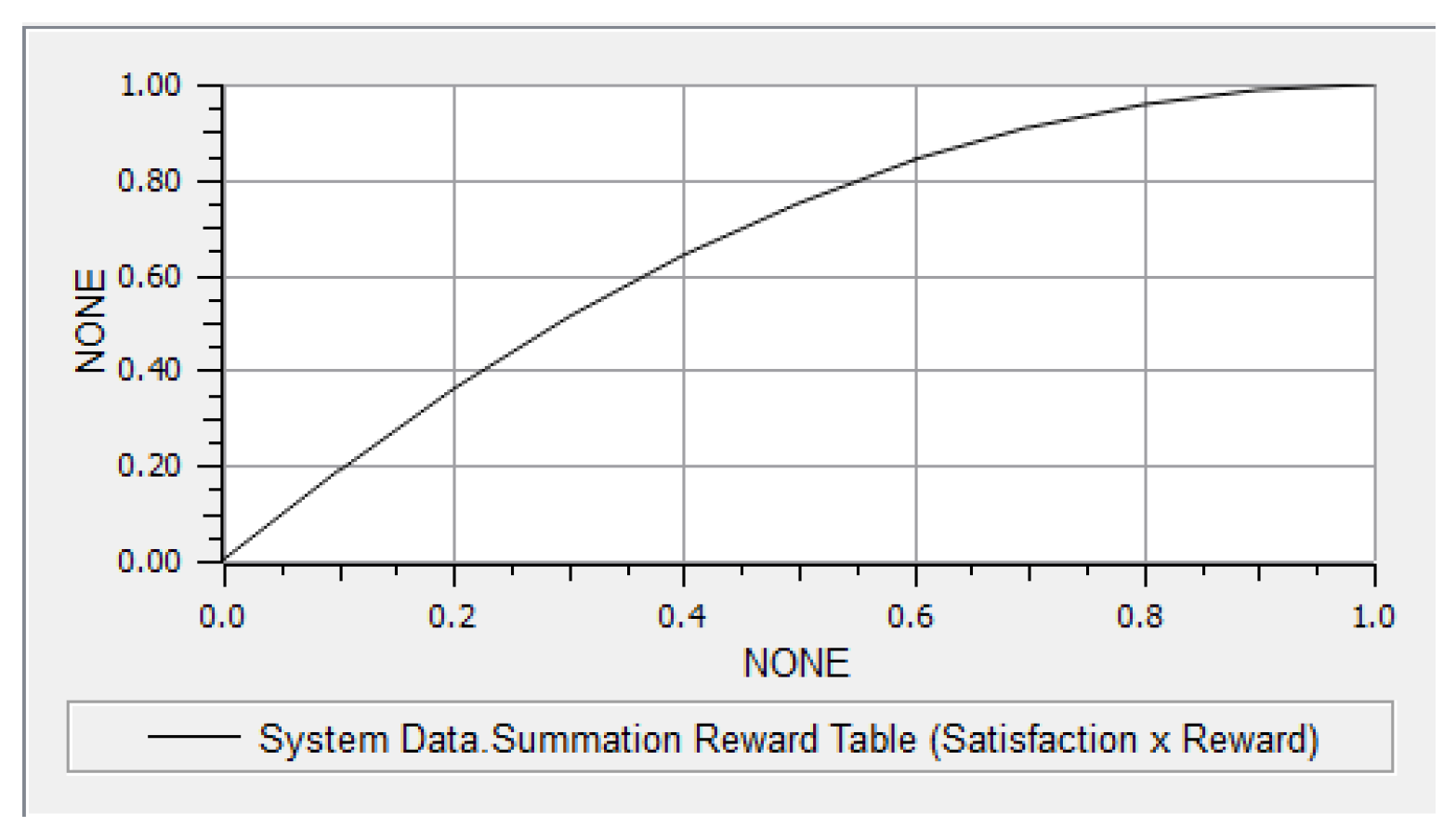
More generally, any concave table may be used. For example, a table can be created for minimizing cubed violations. Tables with more rows may degrade performance (increase run time) and numerical stability. There is a tendency for optimal solutions to be at the discrete values in the table. This may be more noticeable when tables with fewer rows (larger segments) are used. For example, if the reward table only had three rows corresponding to satisfaction values of 0, 0.5 and 1, it might be common to see the solution at a satisfaction of either 0.5 or 1.0. Some experimentation may be required to determine the best table size for a given goal.
It is permissible to use the same reward table for many goals, and this is probably the easiest way to get started. If the results suggest that it may be beneficial to use different tables for some goals, then this can easily be changed. It is also possible to use different reward tables within the same Summation, if desired, by including multiple With Reward Table statements within a single Summation Soft Constraint Set, each referencing a different table slot.
For
Iterative loops can be very useful for adding similar constraints for multiple objects or over multiple timesteps. These iterative loops are added through a For statement. An index variable is assigned to a new value for each iteration of the loop. Inside the loop is one or more Constraint statements which should use the index variable to write a different constraint for each iteration of the loop. The default For loop is as follows:
FOR (NUMERIC index IN <list expr>) DO
ADD CONSTRAINT <boolean expr>
END FOR
where the number of loops is determined by the number of elements in the <list expr>, the NUMERIC label indicates the expression data type of the elements in the <list expr>, and the index is the variable name which will take on the value of each element for use inside the loop. All of these parts of the For statement may be modified. It is also possible to nest a For statement inside another For statement (by replacing the ADD CONSTRAINT statement with another FOR statement) allowing the loops to iterate over two or more variables.
Because Optimization provides a global solution in time, there is no valid notion of Current Timestep; therefore, an important use of FOR loops is to write constraints over all timesteps. Such a FOR loop would have the following form:
FOR (DATETIME index IN @”Start Timestep” TO @”Finish Timestep”) DO
ADD CONSTRAINT Object.Slot[index] == <numeric expr>
END FOR
The time range for the constraint can be modified by changing the expressions in the list expression.
With
A value can be set on a local variable using a With statement. A With statement evaluates an expression and sets the result to a local variable with a given name and type. The statements contained within the With statement may then reference the variable. The default With statement is as follows:
WITH (NUMERIC val = <numeric expr>) DO
ADD CONSTRAINT <boolean expr>
END WITH
If
The addition of a constraint can be made conditional on a boolean expression using an If statement. For example, a constraint might only be applied if the timestep is within a specified season or if a valid value is present within a specified slot on a data object. Without an Else, the statement will do nothing if the boolean expression evaluates to false.
IF (<boolean expr>) THEN
<statement>
END IF
One important difference in the use of an If statement in an Optimization Goal compared to RBS rules is that an If statement in Optimization cannot contain expressions with Optimization variables. For example,
IF (Reservoir.Pool Elevation[@”Start Timestep”] >= DataObject.Max Elevation[]) THEN
would cause the Optimization run to terminate with an error message because Pool Elevation is a variable in the Optimization problem and thus cannot be known when the If statement is evaluated (unless Pool Elevation at the Start Timestep happened to be specified as an input).
Also, If expressions cannot be added within a Constraint statement; however, Constraint statements can be added within an If statement.
If Else
This is similar to the If statement, but an alternative statement will be executed if the boolean expression evaluates to false.
IF (<boolean expr>) THEN
<statement>
ELSE
<statement>
END IF
Else If Branch
Although not a statement by itself, you can add one or more ELSE IF branches to an IF or IF ELSE statement. The ELSE IF is available when the boolean condition or a consequence statement is selected (except when an ELSE consequence statement is selected). An ELSE IF branch is added after the selected branch.
IF(<boolean expr>) THEN
<statement>
ELSE IF(<boolean expr>) THEN
<statement>
END IF
Else Branch
Although not a statement by itself, you can add a single ELSE branch to an IF Statement or ELSE IF statement. This part of the statement will be evaluated when none of the other IF or ELSE IF boolean conditions are true.
IF(<boolean expr>) THEN
<statement
ELSE
<statement>
END IF
Print
A Print statement evaluates its expression and formats the result into a message. The blue message is displayed in the Diagnostics Output window only when the Print Statements diagnostics group is enabled.
PRINT <expr>
where the <expr> is any expression or concatenated expressions which can be fully evaluated and represented as a string. A Print statement can be useful within an If statement to notify the user that system is within a specified condition. See Print Statements in Debugging and Analysis for details about the Print statement.
Notice
A Notice statement posts an orange message to the Diagnostics Output Window regardless of diagnostics settings.
NOTICE <expr>
where the <expr> is any expression or concatenated expressions which can be fully evaluated and represented as a string. See Notice, Warning, and Alert Messages in Debugging and Analysis for details.
Warning
A Warning statement posts a message with a pink background to the Diagnostics Output Window regardless of diagnostics settings.
WARNING <expr>
where the <expr> is any expression or concatenated expressions which can be fully evaluated and represented as a string. See Notice, Warning, and Alert Messages in Debugging and Analysis for details.
Alert
An Alert statement posts a message with an orange background to the Diagnostics Output Window regardless of diagnostics settings.
ALERT <expr>
where the <expr> is any expression or concatenated expressions which can be fully evaluated and represented as a string. See Notice, Warning, and Alert Messages in Debugging and Analysis for details.
Note: The Notice, Warning and Alert statements all have the same behavior. They simply post messages with different colors. This allows you to define messages with three different levels of severity.
Stop Run
A Stop Run statement terminates the run and posts the provided message as a diagnostic error message in red text.
STOP RUN <expr>
A Stop Run might be used if it is known that a certain condition (that can be evaluated prior to the execution of the current goal) will produce an undesirable result, and thus a full Optimization run is not desired. A Stop Run would typically be contained within an If statement.
Timestep References in Optimization
Optimization provides a global solution in time and space (i.e. it solves all timesteps and all objects simultaneously); therefore there is not a valid notion of Current Timestep in Optimization. As such, DateTime expressions such as @”Current Timestep”, @”t” and empty brackets [] (representing current controller timestep on series slots) are not valid in an Optimization Goal Set. Use of these DateTime values will cause the Optimization run to terminate. In order to evaluate an expression or apply a constraint over all timesteps (or a specified range of timesteps) a For loop is used where the index variable is a DateTime set to the values of a list of timesteps in the run. For example, adding a constraint on a reservoir’s Pool Elevation for every timestep could have the following form:
FOR (DATETIME index IN @”Start Timestep” TO @”Finish Timestep”) DO
ADD CONSTRAINT Reservoir.Pool Elevation[index] <= 2,350 “ft”
END FOR
Revised: 08/02/2021