
Provide Approximation Points
When one modeled quantity (slot) is related to one or two other modeled quantities by a non-linear function, then that function must be approximated as one or more linear functions. RiverWare supports three basic ways of approximating a two dimensional function:
• Tangent - the tangent to the function at a given point
• Secant - the line passing through two given points
• Piecewise - several lines connecting points on the function
See Variable Substitution for details about each approximation technique.
Select Optimization methods use their own linearization method that does not depend on the tangent, secant and piecewise approximations. The information in this section does not apply for those methods. In the Optimization Power category, the Power Coefficient method and the Power Surface Approximation method are two such methods. See Power Coefficient and Power Surface Approximation for details. For those methods, a separate set of approximation parameters are entered as described in the section on each method. In the Optimization Tailwater category, the Opt Coefficients Table method uses the same table of coefficients as the corresponding Simulation method to define Tailwater Elevation (i.e. the Simulation method is already a linearized expression of Tailwater). See Opt Coefficients Table for details.
Data Table Slots
Each slot being approximated is related to another slot by a data table. Each row of the table provides a point in the curve describing the relation between the two quantities. In the case of 3-dimensional functions, multiple curves are described in the table.
• 2-D example: Elevation Volume Table, relates Elevation to Storage for a Reservoir.
• 3-D example: Plant Power Table, describes Power as a function of the Operating Head and Turbine Release. The table is organized as several curves, corresponding to Power as a function of Turbine Release for various Operating Heads.
Optimization uses the same data tables that are used in Simulation, or generates the required table automatically based on tables used in Simulation. Thus, a model that runs in Simulation should contain all of required data in data tables to run in Optimization.
LP Param Table Slots
Linear programming parameter tables (LP Param Tables) are specific to Optimization and are required input for an Optimization model. These slots become visible when the Controller is switched to Optimization. The LP Param table slots contain the points to be used when each approximation technique is applied. Setting the values for the LP Param tables can be one of the more challenging aspects of setting up an Optimization model. Setting poor approximation points can result in model infeasibilities that are difficult to debug. Figure 6.1 is an example of a Pool Elevation LP Param table. Basic guidelines for setting LP Param table values follow.
Figure 6.1
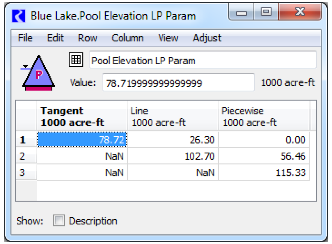
• The Tangent approximation requires a single point. The single approximation point for the tangent approximation should typically be set in the middle of the range of values expected to occur during the current run. The Tangent approximation will overestimate the approximated value for a concave function and underestimate the approximated value for a convex function. See Tangent Approximation for details.
• The Line (Secant) approximation requires two points. They should typically be set near either end of the range of expected values. The Line approximation will overestimate a function at some points and underestimate the function at other points. See Two-point Line Approximation for details.
• The Piecewise approximation requires two or more points. See Piecewise Approximation for details. For piecewise approximation, often it is sufficient to choose the three points used for the Tangent and Secant approximations. In other cases, finer granularity might be required.
Note: Points are entered into the LP Param tables in terms of the independent variables not the dependent variable. For example, the values in the Pool Elevation LP Param table slot are in terms of Storage, not Pool Elevation.
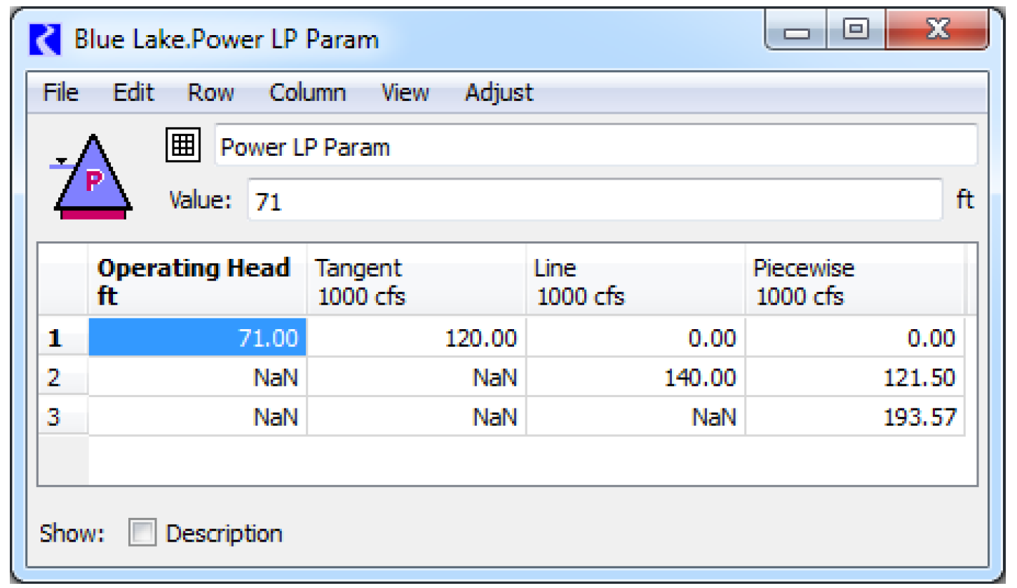
For three-dimensional approximations, the approximation point for the second independent variable (first column in the table) should be somewhere near the middle of the expected operating range. An example of a three-dimensional LP Param table is shown below. For the Power approximation, Turbine Release is the first independent variable and has points set for the Tangent, Line and Piecewise approximations. Operating Head is the second independent variable. A single value is set for Operating Head in the Power LP Param table, and Power is calculated based on this single Operating Head in the Optimization run.
Additional Guidelines
Turbine Capacity Approximation
The Turbine Capacity linearization will always use the Piecewise approximation. Poor Turbine Capacity approximation points can lead to runs that fail in the Post-optimization Rulebased Simulation due to flows that exceed the actual Turbine Capacity in RBS, once the approximation error is removed. When setting the Piecewise points in the Turbine Capacity LP Param table slot, four criteria should be met.
• First, the piecewise curve must be concave. The optimization solution will not behave correctly if the piecewise curve is not concave, and thus the optimization run terminates with an error if the approximation points define a piecewise curve that is not concave.
• Second, the approximation points should cover the full range of operating heads in the Plant Power Table. If the points do not cover the full range, the optimization solution will use a linear extrapolation beyond the highest and lowest approximation points. This can result in excessive approximation error for upper and lower operating heads.
• Third, the piecewise curve defined by the approximation points should never be greater than the curve defined by the Plant Power Table (Auto Max Turbine Q slot). This can result in the optimization solution allowing turbine releases that exceed the actual Turbine Capacity in the post-optimization simulation. In other words, the piecewise curve from the LP Param approximation should always be under the curve defined by the Auto Max Turbine Q table.
• Fourth, the approximation points should be set such that the difference between the piecewise curve and the Auto Max Turbine Q curve is minimized. This reduces the approximation error in the optimization solution. If the difference between the two curves is excessively large, the optimization solution may overly restrict the turbine release to a capacity significantly lower than the actual turbine capacity for the given operating head.
One strategy than can help with picking points for the Turbine Capacity approximation is to plot the Auto Max Turbine Q slot and visually identify reasonable approximation points. The Auto Max Turbine Q slot is automatically populated by RiverWare at the start of the run (even if the run fails). It might be necessary to run the model fist in order to populate the table.
Because the Turbine Capacity linearization always uses the piecewise approximation, it is not necessary to set points for the tangent and line approximations. If values are set for these other two approximations, it will not cause a problem. They will simply never be used. If in doubt, set points for all of the approximations and let RiverWare select the appropriate approximation points to use. If values are missing for an approximation that RiverWare tries to use, the run terminates with an error message notifying the user of the missing values.
Power Approximation
The power approximation tends to be the linear approximation that introduces the most approximation error into the optimization solution. If the Independent Linearizations method is selected in the Optimization Power category, the Power LP Param table is used to define the Power approximation. The table contains an additional initial column for Operating Head in addition to the Tangent, Line and Piecewise columns with Turbine Release values. In the Optimization solution, a single piecewise linear curve for Power as a function of Turbine Release is used. This corresponds to one block of constant head in the Plant Power Table. Operating head is held constant at the value specified in the Power LP Param table. The remaining columns in the Power LP Param table set the Turbine Release for the approximation points.
Typically the Operating Head value in the Power LP Param table should be set to the average Operating Head expected in the run.However, in some cases it might be less problematic to overestimate Power than to underestimate Power. In these cases, it might make sense to set the Operating Head value in the Power LP Param table near the lower end of the expected operating range. This would cause the Optimization solution to underestimate Power, and thus the Post-optimization Rulebased Simulation will calculate a large Power value than the Optimization.
Initialization Rules to Set Approximation Points
n some cases, it might make sense to set the approximation points based on the specific run conditions. For example, for a reservoir that has a large seasonal variation in Pool Elevation, it might not be possible to set Tangent and Line approximation points in the Pool Elevation LP Param table or an Operating Head point in the Power LP Param table that will result in sufficiently small approximation error across all conditions. In these cases, initialization rules can be used to set the approximation points such that the approximation error will be small for the expected operating range of the given run but would be large if operating in a different range in another season. For example, an initialization rule could set the Pool Elevation LP Param Tangent point equal to the initial Storage for the run as shown in Figure 6.2.
Figure 6.2
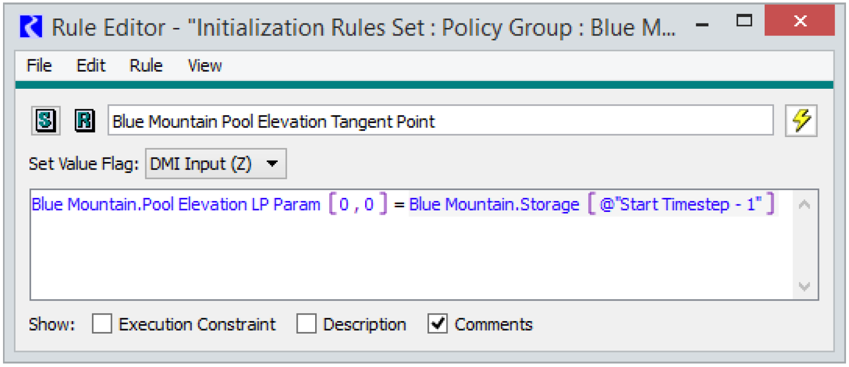
A second rule could set the two Line points to the Tangent point plus or minus some expected delta. In this manner, the approximations will be updated automatically when the model runs, rather than needing to adjust the values manually at the start of each run.
Revised: 01/10/2022