
Limitations of Optimization
The Optimization solution is based on a linear programming solution, and as such, has some inherent limitations as described below.
Optimization License Required
To use the RiverWare Optimization solution, you must have the RiverWare With Optimizer version of the RiverWare license. See www.riverware.org for licensing information.
The license allows to you access the RiverWare Optimization module, which embeds the third-party solver IBM ILOG CPLEX. Additional information about CPLEX can be found in the About RiverWare dialog—from the main RiverWare workspace, select Help, then About RiverWare.
Linear Relationships
All relationships must be linear or piecewise linear. This means that all means that all relationships that are non-linear must be converted to linear or piecewise linear approximations. RiverWare carries out this linear approximation automatically based on approximation points specified by the user. See Linearization, Approximation, and Replacement for details.
Some common non-linear physical processes that must be linearized include the following:
• Power: A function of Operating Head and Turbine Release
• Turbine Capacity: A function of Operating Head
• Tailwater: A function of Outflow and (optionally) Tailwater Base Value (often downstream Pool Elevation)
• Operating Head: A function of Pool Elevation and Tailwater
• Unregulated Spill: A function of Pool Elevation
Linear Constraint Expressions
A corollary to the requirement that all relationship must be linear is that constraint statements can only contain linear expressions. This means that a constraint cannot contain a non-linear combination of variables. Also, to prevent the potential formulation of nonlinear expressions of variables in a constraint, RiverWare does not allow the use of IF/THEN expressions within a constraint statement (even if the IF/THEN expression does not contain a reference to a variable), nor the use of any RPL predefined functions within a constraint statement. Shown below are examples of constraint formulations that would not be valid.
Figure 3.6
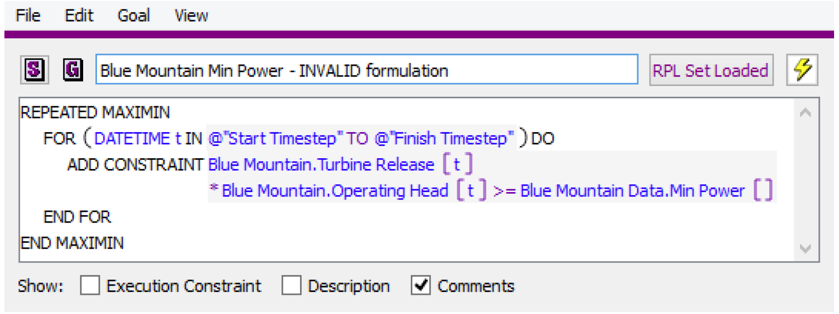
The constraint shown in Figure 3.6 contains a nonlinear combination of two variables, Turbine Release and Operating Head, and would cause the Optimization run to terminate.
Figure 3.7
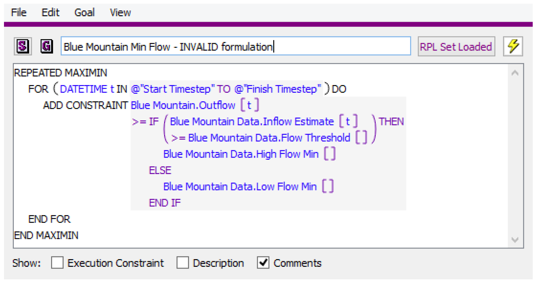
The constraint shown in Figure 3.7 contains and IF/THEN expression within the constraint statement and would cause the run to terminate. This type of logic can be achieved by putting the constraint statement within a WITH statement that carries out the IF/THEN logic. Figure 3.8 is an example of a valid goal.
Figure 3.8
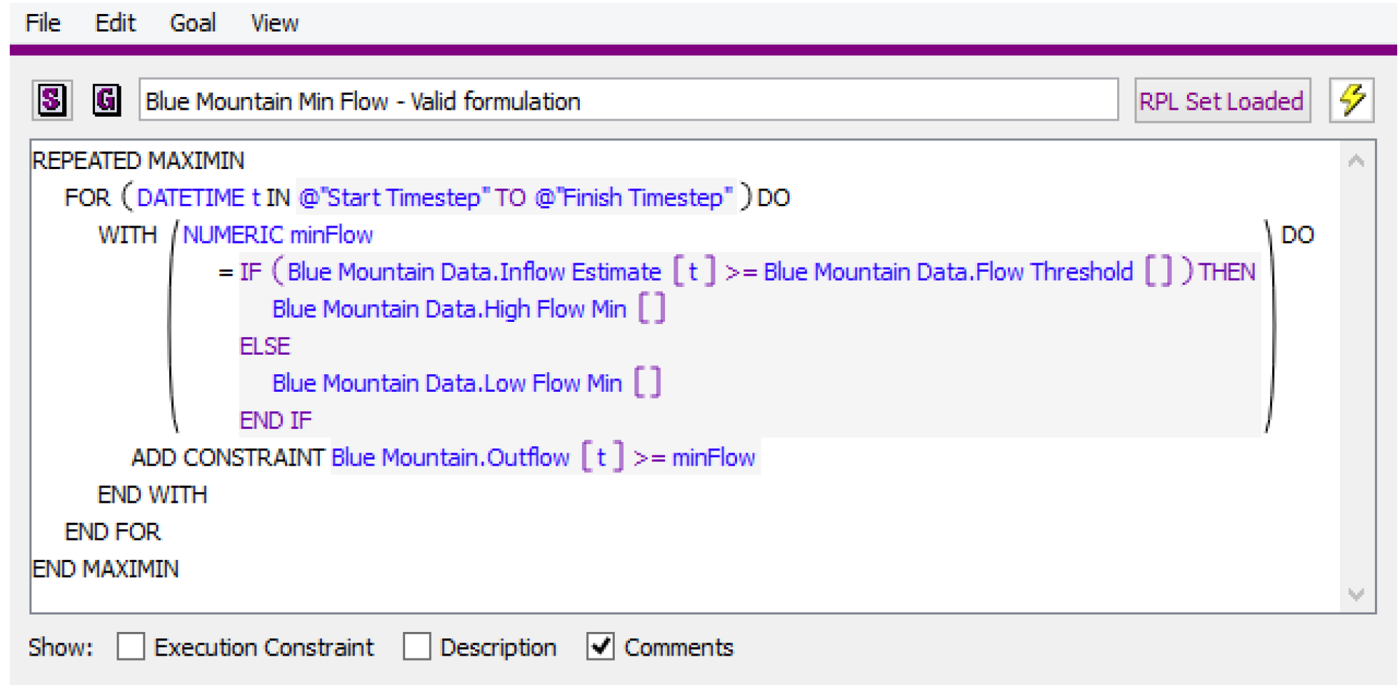
Figure 3.9 is an example of a valid use of IF/THEN logic in an Optimization goal outside of a constraint statement.
Note: In this type of use, the expression in the WITH statement cannot contain a reference to an Optimization variable. Otherwise the expression would return an invalid value, which would cause the goal to terminate without writing any constraints.
Figure 3.9
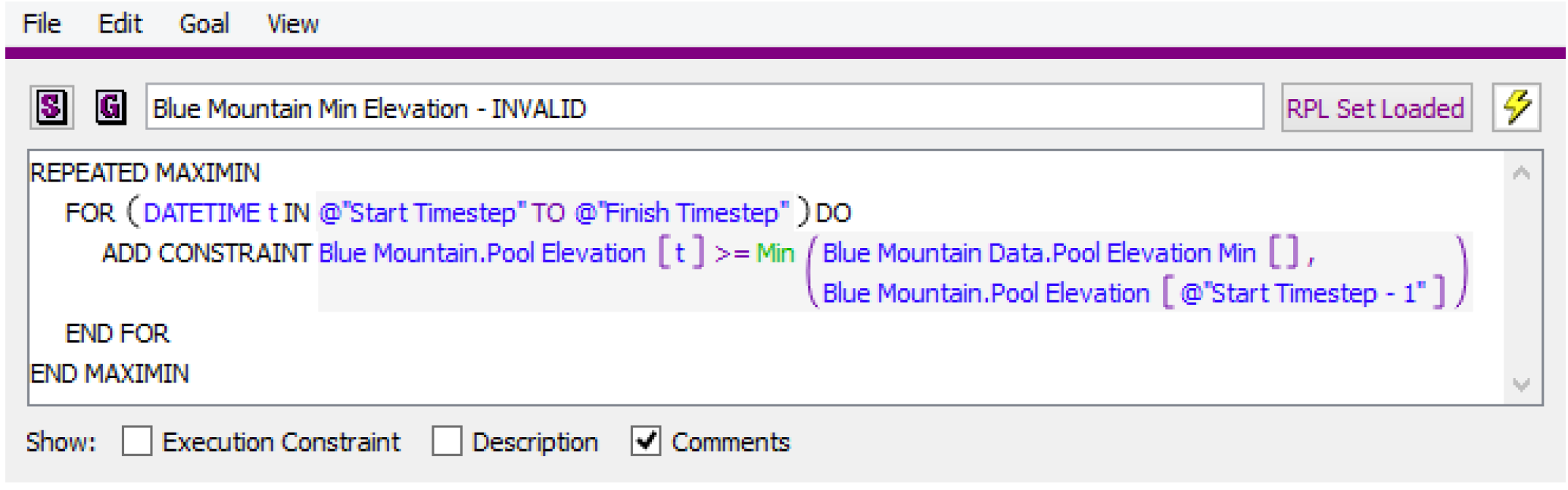
Figure 3.9 contains a RPL predefined function, Min, within the constraint statement and would cause the run to terminate. User-defined functions can be used within constraint statements as long as the functions do not contain nonlinear functions of variables.
Approximation Error
A side effect of the requirement for linear relationships is approximation error. All variables that are linearized will have approximation error in the Optimization solution. Typically the largest and most significant approximation error shows up in the linearization of Power. In the Post-optimization Rulebased Simulation, the rules typically set flow values based on the values for those flow variables from the Optimization solution. Then the objects dispatch and calculate Power and other quantities based on the nonlinear Simulation methods. Therefore the calculation of Power in the Post-optimization RBS, once the approximation error from linearization is removed, will differ from the Power value in the Optimization solution. The Power approximation error tends to be most noticeable when the Optimization policy contains constraints that generation must equal some value (load). In these cases, the Optimization solution will often say that the constraint is 100% satisfied, but the Power calculated in the Post-optimization RBS will not match the constraint value exactly.
Solution Time
The computational requirements of the preemptive linear goal programming solution limit the size of the Optimization problem that can be solved in a reasonable amount of time. For large models (many objects and/or many goals) keeping the run length reasonable typically means limiting the number of timesteps. The definition of reasonable solution time is dependent on the uses of the model, and the user will need to determine what is an acceptable solution time. When determining the upper limit on the number of timesteps, one important point to consider is that the Optimization solution time for a given model does not increase linearly with the number of timesteps, as it generally does for RBS. The relationship between solution time and number of timesteps is typically somewhere between quadratic and cubic. The total solution time is a combination of a number factors, including but not necessarily limited to the following:
• Number of objects (roughly correlates to the number of variables)
• Number of timesteps
• Number of constraints
• Number of goals
• Difficulty of the solution (Objectives that force a lot constraints to be frozen or that have soft constraint violations can take longer to solve.)
• Hardware: Number of available processors, processor speed, memory
Perfect Foresight
The ability of the Optimization solution to look ahead in both time and space (global solution) is one of the benefits of Optimization. Optimization can be used to make sure you do not compromise you ability to satisfy constraints in the future when optimizing for today. However, if not managed appropriately, perfect foresight can be a potential weakness. Because the solution does not inherently put a higher value on one time period over another, in some cases it can exploit the solution to maximize an objective farther into the future, which has a result of degrading the objective in the near term. A common example would be if the value of Energy is somewhat higher later in the run. The solution might save as much water as possible until this higher value period and then generate at max capacity over the high value period. This might be considered a good solution, but in some cases there is more uncertainty about input data farther out in the forecast horizon, and it is not desirable for the solution to over-optimize these future periods at the expense of near term operations. This potential consequence of Optimization’s perfect foresight is important to keep in mind when considering the appropriate run horizon for an Optimization model.
Limited Objects and Method Selections
Not all object types are supported by Optimization. Additionally, only a subset of Simulation user methods can be used in conjunction with Optimization. See Optimization Objects and Methods for a complete listing of the available objects and methods. When creating a model that will be used for Optimization, it is important to make Simulation method selections that are compatible with Optimization.
Debugging
The Optimization solution is generally more difficult to debug than Rulebased Simulation. Because it is a global solution, there is typically not a single cause for a bad output or odd result. It can be the combination of multiple constraints and input data at multiple locations and multiple timesteps. Often the solution can be exploited to improve some objective function if it is not properly constrained, resulting in unrealistic or undesirable operations. In these cases it can be difficult to determine what exactly is contributing to the undesirable result. See Debugging and Solution Analysis for descriptions of tools that can assist in debugging the Optimization solution.
Revised: 01/10/2022