
Algorithms
Following is a description of the available algorithms.
Bisection
The Bisection algorithm is the most basic and most robust algorithm implemented. All other algorithms fall back to the bisection if the individual run does not succeed. In Bisection, the minimum and maximum yield is tried first. Then the min and max are averaged or bisected to find the intermediate yield and a run is made with that value. After the third run, the algorithm decides if the yield is too high or too low and modifies the upper or lower bound as appropriates and bisects again. This procedure continues until the solution is found. It is robust as the min and max yields are tried first to bound the solution. No additional information on the reservoirs or physical processes are used, so it is often the simplest to get working. It can be slow as it uses a brute force approach; no information on the processes are used to estimate the next yield to try.
Heuristic A
In Heuristic A, first the minimum, then the maximum yields are tried. Then the average of those two yields is tried. If this third and subsequent yield estimate is too high, meaning the minimum level difference is negative, the bisection method will be used as described above. If the minimum level difference is positive the following approach will be taken to compute the next yield.
Assume that we have completed a simulation with a yield which resulted in a positive minimum level difference, i.e. the reservoir is above the bottom of conservation pool throughout the run. In this case, we have underestimated the yield. Examining the results from the simulation, we can find the dates of the drawdown period defined as the last date when the reservoir was full (at the top of the conservation pool) to the date of the minimum level difference. If we had guessed the correct yield then the drawdown period would have ended in a minimum level difference of zero, but we know that we underestimated the diversion because there is water remaining in the conservation pool at the end of the drawdown period. To exactly drain the conservation pool during the drawdown period, we would have needed to divert additional storage equal to the volume of the conservation pool at the minimum level difference date as well as enough to compensate for the reduced evaporation which would result from lower elevations over the drawdown period.
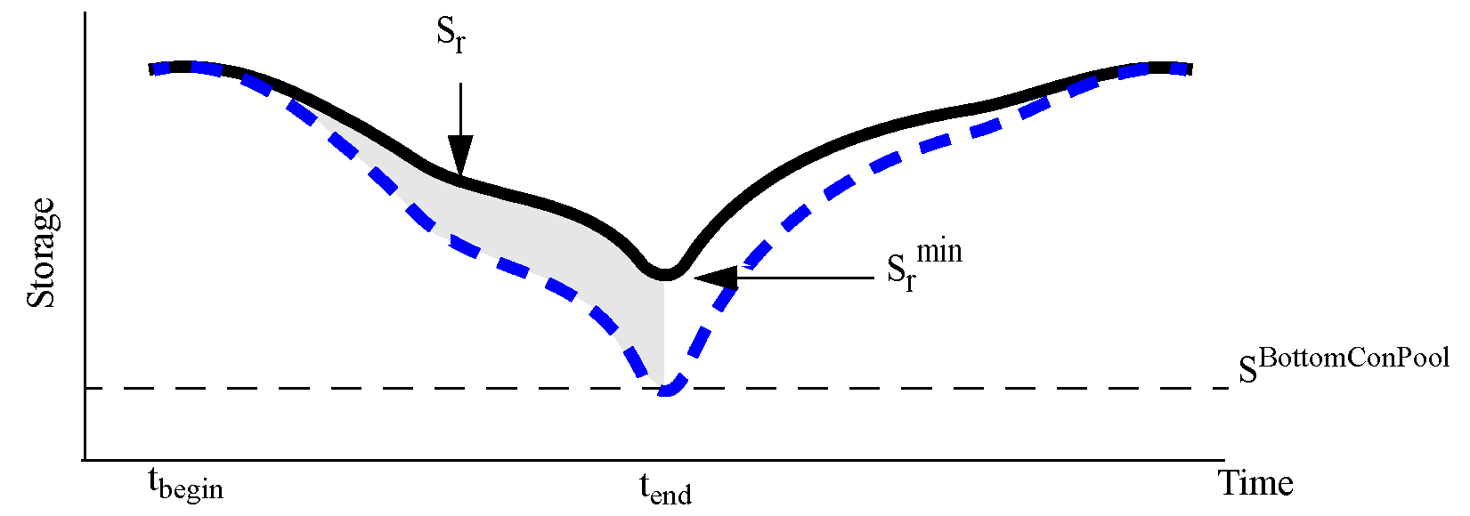
Figure 5.7 shows a plot of storage versus time for this situation. In this figure, the curve Sr is the storage produced from the previous run. Additional water must be released to lower the pool to the bottom of conservation pool. The shaded area is the volume of water that must be released to scale the solid black curve to reach the bottom of conservation pool. This would produce a curve similar to the dotted blue curve.
Figure 5.7 Plot of a sample drawdown period
This analysis motivates Equation 5.1 for using the results from one run to choose a yield which will lead to a minimum level difference of zero in the next run.
(5.1) 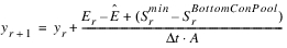
where:
– y = average yield
– r = run number, r is the previous run, r+1 is the next run
– Smin = minimum storage that occurred (i.e., storage at minimum level difference date)
– SBottomConPool = storage corresponding to an empty conservation pool
– A = average yield distribution factor over the drawdown period. The yield may be distributed to the Reservoir Diversion based on factors representing the percentage/fraction of the average yield. These factors are stored in the Distribution Yield periodic slot and must average to 1.0 over the course of a year. Otherwise an error is issued and the run stops. Because of this distribution, the average of the yield over the critical period may not be 1.0. In this equation, we divide by the average distribution factor over this period to ensure that we are still dealing with average yield.
–  = Duration of the drawdown period, tbegin to tend
= Duration of the drawdown period, tbegin to tend – E = Total evaporation over drawdown period
– Ê = Estimated total evaporation that would occur over the drawdown period if the true yield were released. Increasing the yield from the last run will lead to lower storage values over the drawdown period, which will in turn lead to a lower evaporation over the drawdown period. We estimate Ê by computing the evaporation which would result from a drawdown period whose Storage (S) is like the previous run’s Storage, except it is scaled so it reaches the bottom of the conservation pool at the end of the drawdown period (i.e., the blue dotted line in the figure). The estimate for the storage during the drawdown period when we are using the true yield is calculated using Equation 5.2.
(5.2) 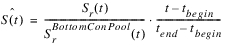
where:
– tbegin = the begin date of the drawdown period
– tend = the end date of the drawdown period
Then we can use this along with the method for computing evaporation as a function of storage, Evap(S(t)), to compute the total estimated evaporation over the drawdown period using Equation 5.3.
(5.3) 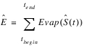
Heuristic B
In Heuristic B, the minimum and maximum yields are computed to bound the solution, but no runs are made with the values. Instead the average of them is used on the first run (If the Reservoir Data for Bisection.Initial Yield to Try is not specified). Then after each successful run, regardless of whether the minimum level difference is positive or negative, the  is computed using Equation 5.1 and used on the next run. On unsuccessful runs, a bisection is used.
is computed using Equation 5.1 and used on the next run. On unsuccessful runs, a bisection is used. Choosing a Method
Table 5.1 summarizes the strengths and weaknesses of each algorithm. This is particularly important for long model runs where any extra runs means hours of computations. own.
Algorithm | Strengths | Potential Weakness |
|---|---|---|
Bisection | Most robust and easy to understand. Requires the least amount of effort if evaporation or other physical processes are involved. | Potentially slow as runs are made to ensure the upper and lower bounds encompass the solution point. Also slower as it just keeps going until a solution is found. No information from the run is used to guide the next run. |
Heuristic A | Potentially faster than bisection. Like Heuristic B, information from this run can be used to guide the trial in the next run. | Because the heuristic is only used for positive minimum elevation differences, the search may be close to the final solution but then has a negative minimum elevation, so then uses bisection and jumps away from the final solution. |
Heuristic B | Faster; the first two runs for each reservoir are skipped and the estimated yield is always used for the next run. | Because the upper and lower bounds are not tried first, the solution could be outside the bounds and would not be caught until hitting max iterations and/or attempting to converge on the bound. |
Revised: 01/10/2022