
Soft Constraints and Derived Objectives
In RiverWare, operational policy constraints created by the user are typically added to the optimization problem as prioritized soft constraints. (Constraints defining the physical characteristics of the system are automatically added to the optimization problem by RiverWare as hard constraints; see Physical Constraints for details.) RiverWare automatically converts the soft constraints at each priority into a derived objective to maximize the satisfaction of the soft constraints (minimize violations). This is done to prevent an infeasible problem in the case that it is not possible to satisfy all constraints. If it is not possible to fully satisfy all constraints at a given priority, the solution will get as close as possible, rather than return an infeasible solution. The next section provides a simple example with two variables to illustrate the conceptual use of prioritized soft constraints. This is followed by a simple example from a water resources management context. See Satisfaction Variables in Soft Constraints for details about how soft constraints are defined. See Derived Objectives for details about how derived objectives are formulated.
Prevent Infeasibilities
Two-dimensional Example
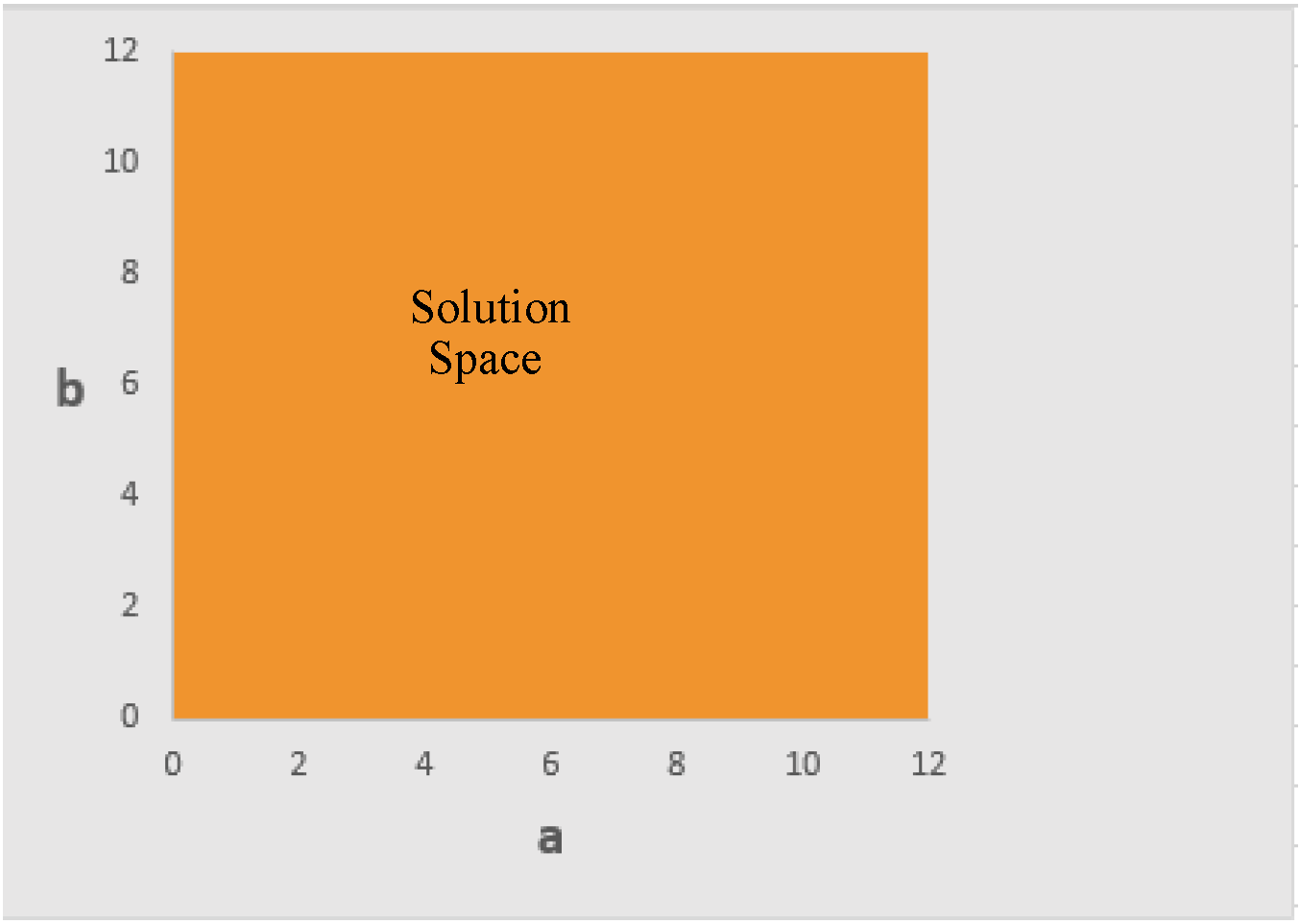
To illustrate the conceptual use of prioritized soft constraints to prevent infeasibilities, assume an optimization problem with two variables, a and b. The variables have the following formal bounds.


Figure 2.3 illustrates the solution space given these bounds.
Figure 2.3
The problem has the following soft constraints and objectives in order from highest priority to lowest priority.
1. Soft Constraint: 
2. Soft Constraint: 
3. Soft Constraint: 
4. Objective: Maximize 
5. Objective: Maximize 
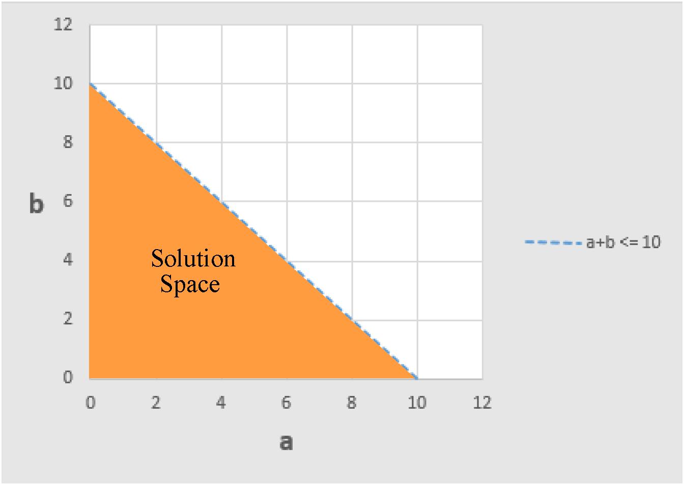
At priority 1, adding the constraint  reduces the solution space; see Figure 2.4.
reduces the solution space; see Figure 2.4.Figure 2.4
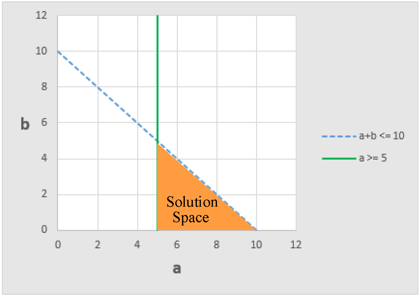
At priority 2, the constraint  further reduces the solution space; see Figure 2.5.
further reduces the solution space; see Figure 2.5.Figure 2.5
Now when we get to priority 3, we can see that the constraint  cannot be satisfied without violating one of the two higher priority constraints. If the constraints were all hard constraints, the problem would be infeasible, and there would be no solution. Using soft constraints, the solution gets as close as possible to satisfying the constraint. It does this in a way that minimizes the violation of the priority 3 constraint in a manner that does not compromise the satisfaction of the two higher priority constraints; see Figure 2.6.
cannot be satisfied without violating one of the two higher priority constraints. If the constraints were all hard constraints, the problem would be infeasible, and there would be no solution. Using soft constraints, the solution gets as close as possible to satisfying the constraint. It does this in a way that minimizes the violation of the priority 3 constraint in a manner that does not compromise the satisfaction of the two higher priority constraints; see Figure 2.6. Figure 2.6
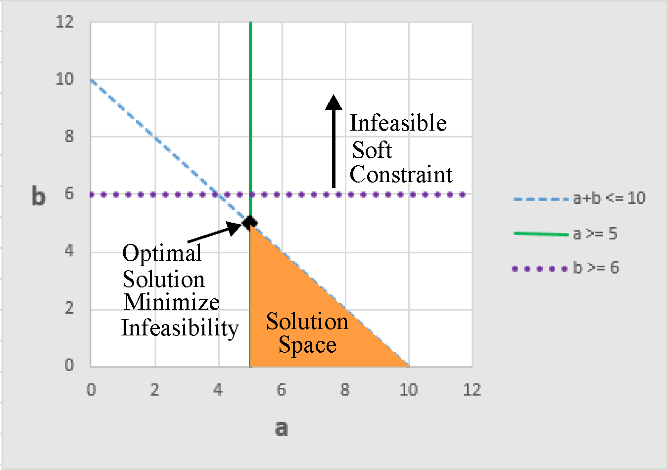
In this case, priority 3 removes all degrees of freedom from the solution. All of the constraints are frozen, and there is only one optimal solution.


With no degrees of freedom remaining, the two objectives can do nothing to affect the solution.
Goal Programming With Many Dimensions
In the two dimensional examples above, we saw that a soft constraint may have one of several possible effects on the solution space:
• Cut away a portion of the 2-d solution space, leaving a smaller 2-d area as the new solution space
• Limit the solution to a 1-d line segment
• Pick a 0-d solution, a single point, which is a vertex
A soft constraint could also have no effect because it does not reduce space of feasible solutions.
If we extend the goal programming solution to a problem with three variables (three dimensions), the initial solution space is represented by a 3-d polyhedron. A soft constraint may have one of several possible outcomes:
• Cut away a portion of the 3-d polyhedron, leaving a smaller 3-d polyhedron as the new solution space
• Limit the solution to a face of the polyhedron, which is a 2-d polyhedron
• Limit the solution to a 1-d line segment on the polyhedron
• Pick a 0-d solution, a single point, which is a vertex of the polyhedron
• No effect because it does not reduce the polyhedron of feasible solutions
Goal programming in higher dimensions is similar. In n dimensions, if a constraint has an effect, it may result in a smaller polyhedron with n or fewer dimensions.
Goal programs used in a water resource management context typically have many dimensions. Each physical component (e.g. Reservoir Storage, Reservoir Outflow, Reach Outflow) at each timestep is an individual variable in the problem. Additional decision variables that do not represent physical components of the system may also be included at each timestep (e.g. Energy Value). This results in a solution space represented by a polyhedron in many dimensions.
Note: RiverWare only adds the variables to the problem that are necessary based on the specified policy. See Constraints Define Variables and Physical Constraints for details. In addition, any quantities that are known inputs are included in the problem as numeric values, not as variables. For example, the Inflow to the upstream reservoir in a basin might be provided as an input. In this case, the Inflow would not be a variable. The numeric inputs would get incorporated into problem as appropriate, in mass balance constraints for example.)
Water Resource Management Example
To illustrate how goal programming applies in a water management context, consider the following simple example.
A reservoir is modeled for a single timestep with a length of one day. The initial storage of the reservoir is 50,000 acre-ft, and the inflow over the timestep is an input at 2,000 acre-ft/day. (Assume a single inflow, a single outflow and no other gains or losses.) The reservoir has the following operational policy in priority order, highest priority to lowest.
1. Minimum Storage Constraint: 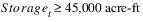
2. Minimum Outflow Constraint: 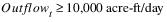
3. Maximize Storage Objective: Maximize 
The priority 1 constraint can be fully satisfied and guarantees that the Storage will not go below 45,000 acre-ft when solving for the later priorities.
The priority 2 constraint cannot be fully satisfied without drafting the reservoir to 42,000 acre-ft, but priority 1 already guaranteed that the reservoir would not go below 45,000 acre-ft. So priority 2 will get as close as possible to meeting the Minimum Outflow by setting the Outflow to 7,000 acre-ft/day. This will freeze both constraints as follows:
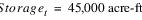
In this case there are no degrees of freedom remaining for the priority 3 objective, so it will do nothing to the solution. If the constraints at priorities 1 and 2 were added as hard constraints, the problem would be infeasible, and there would be no solution. Using soft constraints provides a solution that gets as close to the constraints as possible based on their priorities.
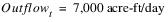
Now assume that the inflow over the timestep is 7,000 acre-ft/day. Both constraints could be fully satisfied, and the objective at priority 3 would result in the following solution.
In practice, optimization problems for a water management context are far more complex, spanning many timesteps, multiple objects (physical features of the basin) and many operational policy constraints and objectives. The initial solution space is a polyhedron of many dimensions. In those contexts, the general conceptual approach is the same as for this example: at each priority get as close to satisfying the constraints as is possible (maximize satisfaction) without degrading any of the higher priority constraints or objectives. However there are multiple possible approaches to maximize satisfaction. The use of soft constraints and derived objectives to maximize soft constraint satisfaction in the RiverWare Optimization solver are described in more technical detail in the following sections.
Satisfaction Variables in Soft Constraints
This section describes how satisfaction variables are introduced to formulate soft constraints. The following section describes how those satisfaction variables are included in a derived objective to maximize the soft constraint satisfaction (minimize violations).
In RiverWare, soft constraint violations, vi, are scaled from 0 to 1 where 1 corresponds to the maximum violation from a higher priority constraint or bound. For performance reasons, the RiverWare Optimization solution actually uses a formulation based on satisfaction rather than violations.

It then maximizes satisfaction, where 1 corresponds to fully satisfied, and 0 corresponds to doing no better than the previous bound.
As an example, assume a reservoir has the following high priority minimum flow constraint.
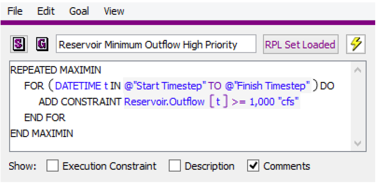
(Technically this would translate to multiple constraints, one for each timestep.) Then assume that at a lower priority a more restrictive target minimum outflow is added.
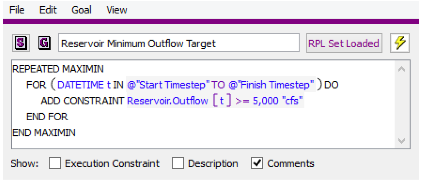
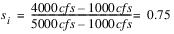
Now assume that the high priority minimum flow constraint of 1,000 cfs was fully satisfied on all time steps, but on one time step it was only possible to get an outflow 4,000 cfs due to some other high priority constraints and low inflows. The lower priority target minimum outflow would not be fully satisfied. The satisfaction, si, for that particular constraint would be 0.75. 4,000 cfs is 75% of the way from the old lower bound of 1,000 cfs to the new constraint value of 5,000 cfs.
For a greater-than-or-equal-to constraint containing only a single variable, this can be expressed as:
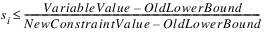

In the above example,
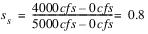
Now assume that the high priority constraint setting a minimum of 1,000 cfs did not exist, and thus the constraint using 5,000 cfs was the first constraint with this left-had-side formulation. In this case, the OldLowerBound would be taken from the Lower Bound set on the variable (slot configuration); see Variable Bounds for details. Assume that the slot Lower Bound was 0 cfs. Then the satisfaction would be
More generally, a soft constraint is defined as

or


where each xn is an optimization variable in the constraint. Each an is a numeric coefficient on the corresponding variable, b is the right-hand-side numeric constraint value, and OldBound is the previous limit for the right-hand-side either from a higher priority constraint of the same form (same left-hand-side) or based on the slot bounds if there is not a higher priority constraint with the same LHS.
Note: Internally, RiverWare always rearranges all constraints to have this same canonical form, with the sum of variables and their coefficients on the LHS and all constant numeric values combined in a single RHS value.
For every priority that contains soft constraints, RiverWare adds the constraints in this form, using satisfaction variables, to Optimization problem. It will then solve the Optimization problem at that priority with a derived objective to maximize the satisfaction. The derived objective that RiverWare automatically creates to maximize the value of the satisfaction variables is described in the following section.
Derived Objectives
For all priorities that contain soft constraints, RiverWare automatically generates an objective to maximize the satisfaction of the soft constraints and then solves the Optimization problem at that priority to maximize the derived objective with the new soft constraints added. The manner in which satisfaction is maximized depends on which type of derived objective is selected. Each of the derived objectives are described in the following sections. See Soft Constraint Set for details about how to select the derived objective to use.
There are three general types of derived objectives in RiverWare: Summation, Single Maximin and Repeated Maximin. In addition Summation with Reward Table (Reward Function) is described here as a fourth type of derived objective, though technically it is implemented by adding a “With Reward Table” statement within a Summation derived objective. See With Reward Table for details.
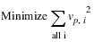
Summation
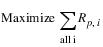
The Summation derived objective includes a separate satisfaction variable in each constraint added to the Optimization problem at the current priority p. The objective is then to maximize the sum of all of the satisfaction variables added at that priority.
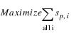
where there is one satisfaction variable, sp,i, for each constraint i added at the current priority p.
After maximizing the derived objective, the objective value is frozen so that the objective (satisfaction) is not degraded by lower priority objectives. Conceptually the following constraint is added to the Optimization problem

where zp is the value from maximizing the derived objective. Technically this constraint does not get included, but the equivalent of adding this constraint is carried out by freezing select constraints and variables. See Freezing Constraints and Variables for details about freezing constraints and variables.
The potential downside of the Summation approach is that it can tend to place all of the deviation on one or just a few constraints. For example, if a minimum flow constraint cannot be met for every timestep, it might minimize the total violation by satisfying the constraint at all but one timestep and putting a very large violation on that one timestep. Typically, this is not the preferred solution in a water resources context.
Single Maximin
The Single Maximin derived objective applies the same satisfaction variable, sp, for all constraints added at priority p. The objective is then to maximize the value of that single satisfaction variable.

Instead of minimizing the total violation, this approach will minimize the single largest violation (formally it maximizes the minimum satisfaction). This prevents a single, very large violation by spreading the violation out over multiple variables or timesteps.
Conceptually, the following constraint is added to the Optimization problem to freeze the satisfaction.

where zp is the value from maximizing the derived objective. Technically this constraint does not get included, but the equivalent of adding this constraint is carried out by freezing select constraints and variables. The solution will freeze all constraints that are limiting the satisfaction if sp is less than 1. These are the constraints with the largest violation. See Freezing Constraints and Variables for details about freezing constraints and variables.
The potential downside of the Single Maximin approach is that it does nothing to improve the satisfaction of the remaining constraints that are not frozen. There might be other constraints introduced at priority p that could have a higher satisfaction that the limiting constraints, but this approach does nothing to enforce that higher satisfaction when moving on to solve at lower priorities. It only guarantees that they will have the same satisfaction as the least satisfied constraint. This issue is addressed by the next type of derived objective, Repeated Maximin.
Repeated Maximin
The Repeated Maximin approach begins with the single maximin. A single satisfaction variable, sp,1, is applied for the first iteration for all constraints added at the current priority p, and it solves the Optimization problem with an objective to maximize the satisfaction variable (minimize the largest violations). It then conceptually freezes the satisfaction variable (satisfaction of the constraints with the largest violation). It also freezes all constraints that are limiting the satisfaction if sp,1 is less than 1. These are the constraints with the largest violation. (See Freezing Constraints and Variables for details about freezing constraints.) It then adds a new satisfaction variable, sp,2, for all remaining constraints and solves to minimize the next largest violation (technically maximize the next smallest satisfaction). It repeats this process until either all violations have been minimized (all constraints added at the current priority p have been frozen) or all remaining constraints can be fully satisfied (sp,i) equals 1.
While sp,i-1 < 1

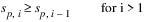
where sp,i is a single satisfaction variable applied to all constraints added at the current priority p that have not yet been frozen prior to the ith Repeated Maximin iteration.
If it is possible to fully satisfy all constraints added at the current priority p (i.e. sp,i = 1), there will only be a single iteration. In this case there may not be any constraints frozen, dependent on whether the goal forced any constraints to their limits.
When it is not possible to fully satisfy all constraints at a given priority, the Repeated Maximin approach tends to spread out deviations as evenly as possible, which is often the desired solution in a water resources context. We recommend Repeated Maximin as the default approach for most soft constraints. It is relatively easy to change to one of the other types of derived objectives later if this is desirable.
The potential downside of the Repeated Maximin approach is that in some cases it can require numerous iterations when it is not possible to satisfy all constraints. Depending on the size of the model this can cause a significant increase run time. The Summation approach always requires only a single solution at each priority, so it tends to be faster, but it does not, in general, provide the same solution quality as Repeated Maximin. In some cases, a reasonable balance between solution quality and run time can be provided by applying the Summation with Reward Table approach as described in the next section.
Summation with Reward Table
Summation with Reward Table is a special case of the Summation derived objective. Rather than summing all satisfaction variables at a given priority equally, this approach applies a reward function to each of the satisfaction variables. Typically this approach is used to penalize larger violations more than smaller violations (greater reward for higher satisfaction). For example, a common approach is to minimize the sum of squared violations. This tends to smooth out large violations by spreading them out over multiple time steps rather than concentrating large violations on a few time steps. Applying the appropriate reward function can often produce a result that compares to the Repeated Maximin solution in terms of solution quality but has the benefit of only requiring a single solution at the given priority and can therefore be much faster.
Note: Technically, the Summation with Reward Table approach is implemented by adding a With Reward Table statement within a Summation derived objective. See With Reward Table for details on implementing Summation with Reward Table.
A reward table is used to apply a piecewise function to the satisfaction variables within a Summation objective. Instead of using the standard Summation derived objective for maximizing satisfaction, the derived objective becomes
where R is the reward function for the satisfaction variables.

The reward table slot has two columns. The first column contains satisfaction values. The second column contains the corresponding reward values. The values in both columns must be between 0 and 1. The reward table must be concave. (Reward must be a concave function of Satisfaction.)
Details of the general formulation of the Summation with Reward Table derived objective are given below, followed by an example that minimizes the sum of squared violations.
The following constraint is added that defines the satisfaction Sp,i of constraint i introduced at priority p as the sum of all piecewise segments.

where xp,i,j is the length ( ) of each segment j. The number of segments is defined by the Reward Table (# segments = # rows - 1). The maximum length of each segment is constrained by the satisfaction values sp,i,j entered in the first column of the Reward Table.
) of each segment j. The number of segments is defined by the Reward Table (# segments = # rows - 1). The maximum length of each segment is constrained by the satisfaction values sp,i,j entered in the first column of the Reward Table.
The first row in the table is indexed as row 0. The slope for each segment mp,i,j is calculated as
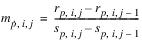
where each rp,i,j is the value in the Reward column of the Reward Table corresponding to the satisfaction sp,i,j.
The objective maximizes the total reward Rp, which is defined as follows.
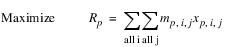
An example is provided below for a reward table that corresponds to minimizing the sum of squared violations
Example 2.1 Example Reward Table: Minimize the Sum of Squared Violations
Conceptually the desired derived objective is to minimize the sum of squared violations of all constraints introduced at the current priority p.
where vp,i is the violation of constraint i introduced at the current priority p. Violations are scaled from 0 to 1, where 1 corresponds to the maximum violation based on a higher priority constraint or variable bound. Thus an equivalent objective to minimize the sum of squared violations is
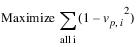
For performance reasons, the RiverWare Optimization solution maximizes satisfaction variables rather than minimizing violations. See Satisfaction Variables in Soft Constraints for details about how the satisfaction variables are defined.

The maximize objective then becomes
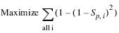
Table 2.1 shows how this can be approximated by a piecewise linear function that linearizes the function in 10 discrete segments.
vi | vi2 | si | 1 - vi2 |
|---|---|---|---|
1.0 | 1.00 | 0.0 | 0.00 |
0.9 | 0.81 | 0.1 | 0.19 |
0.8 | 0.64 | 0.2 | 0.36 |
0.7 | 0.49 | 0.3 | 0.51 |
0.6 | 0.36 | 0.4 | 0.64 |
0.5 | 0.25 | 0.5 | 0.75 |
0.4 | 0.16 | 0.6 | 0.84 |
0.3 | 0.09 | 0.7 | 0.91 |
0.2 | 0.04 | 0.8 | 0.96 |
0.1 | 0.01 | 0.9 | 0.99 |
0.0 | 0.00 | 1.0 | 1.00 |
The reward table entered in RiverWare is taken from the last two columns, as shown in Figure 2.7 and Figure 2.8.
Figure 2.7
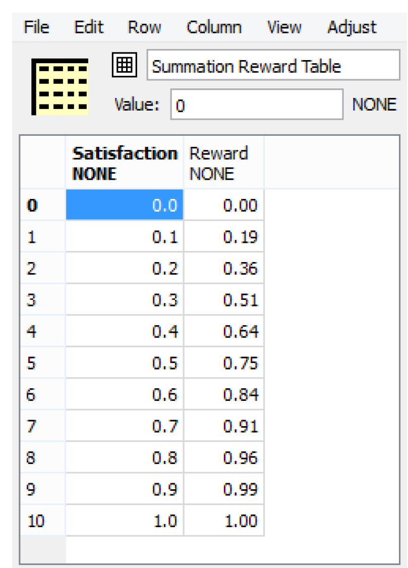
Figure 2.8
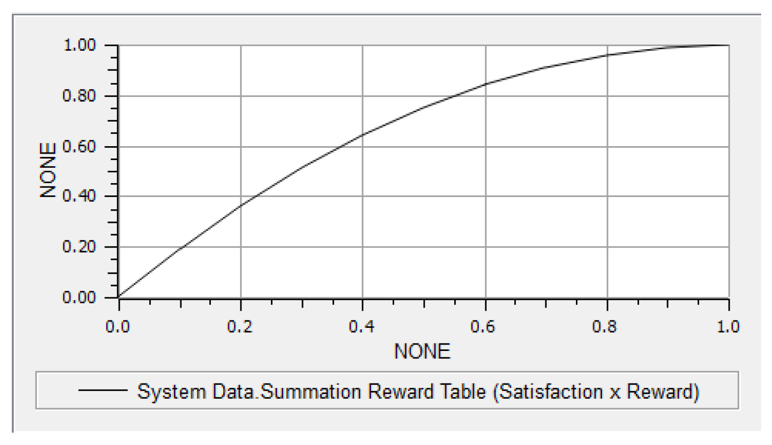
More generally, any concave table may be used. For example, a table can be created for minimizing cubed violations. Tables with more rows may degrade performance (increase run time) and numerical stability. There is a tendency for optimal solutions to be at the discrete values in the table. This may be more noticeable when tables with fewer rows (larger segments) are used. For example, if the reward table only had three rows corresponding to satisfaction values of 0, 0.5 and 1, it might be common to see the solution at a satisfaction of either 0.5 or 1.0. Some experimentation may be required to determine the best table size for a given goal.
Revised: 08/04/2020