
Optimization Variables
An optimization problem technically consists of a set of equations that include linear combinations of optimization variables. The following sections describe how those variables are defined.
Slots and Variables
In RiverWare, some Optimization variables are directly related to slots. Other variables are related to slots by a linearized expression. Still other variables have no relation to slots, and some slots have no relation to variables. RiverWare decides automatically which variables to add to the Optimization problem based on what is referenced in the Optimization Goal Set.
All slots that are related to Optimization variables, either directly or by linearized expressions, are series slots. These could be multislots or agg series slots, which are forms of series slots. In the case of agg series slots, each column corresponds to a separate variable.
Note: While it is common to refer to a slot and a variable synonymously, technically each individual variable within the Optimization problem, is associated with a single slot at a single timestep.
Slots as CPLEX Variables
Some slots are related directly to variables. For example, Outflow and Storage on a reservoir object are common variables. Each of these slots at each timestep corresponds directly to an individual variable in the Optimization problem. Some additional examples of slots that are directly related to variables are provided below for various objects.
• Canal: Flow1
• Confluence: Outflow
• Reach: Outflow
• Reservoir: Outflow, Spill, Storage, Release, Diversion, Cumulative Storage Value
• Power Reservoir: Turbine Release, Pumped Storage Outflow
• Slope Power Reservoir: Qc1, Level Storage, Pool Elevation
Linearized Slots
In some cases slots correspond to a linear combination of variables. One example is Power. The manner in which Power is linearized depends on the method selected in the Optimization Power category. With the commonly used Independent Linearizations method, Power is defined by a piecewise linear function of Turbine Release. Each individual variable, or piece, is multiplied by the slope of that segment of the power curve. The sum of the pieces is equal to the total Turbine Release. Examples of slots that correspond to linearized expressions of variables are provided below.
• Canal: Delta Elevation, Elevation 1, Elevation2, Flow 2
• Confluence: Inflow 1, Inflow 2
• Reach: Inflow
• Reservoir: Canal Flow, Energy In Storage, Inflow, Pool Elevation, Spill Cost, Spilled Energy, Spilled Power
• Power Reservoir: Best Turbine Flow, Energy, Future Value Used Energy, Hydro Capacity, Operating Head, Power, Pumped Storage Inflow, Spill Capacities, Tailwater Base Value, Tailwater Elevation, Turbine Capacity
• Pumped Storage Reservoir: Pump Capacity, Pump Energy, Pump Power, Pump Q Capacity
• Slope Power Reservoir: Backwater Elevation, Inflow 2, Wedge
Variables Unrelated to Slots
Some variables have no relation to a slot in RiverWare. For example, the satisfaction level of each Repeated Maximin iteration or the satisfaction of each constraint in a Summation derived objective is added to the Optimization problem as a variable. See Satisfaction Variables in Soft Constraints for details about how satisfaction variables are defined.
Slots Unused by Optimization
Some slots apply to Simulation only and do not get used by the Optimization solution. For example, the Total Inflows and Inflow Sum slots on a Reservoir object do not get used by the Optimization solution. The components that make up Total Inflow and Inflow Sum in Simulation are expressed as individual variables and are incorporated into the mass balance constraint for the Reservoir, but there is not a separate Total Inflows or Inflow Sum variable that is defined. (Total Inflow and Inflow Sum will get calculated in the final results from the Post-optimization Rulebased Simulation.)
Constraints Define Variables
In an optimization run, the controller executes the user’s policy which consists of a series of constraints and objectives. RPL expressions add constraints to the current optimization problem, cause the problem to be solved with a given objective, or freeze some aspects of the current problem solution. When the policy refers to the value of a slot at a given timestep, RiverWare automatically adds constraints to the problem which define the variable associated with the slot value at that timestep. As an example, assume the following goal is at priority 1 in the Goal Set. See Figure 4.12.
Figure 4.12
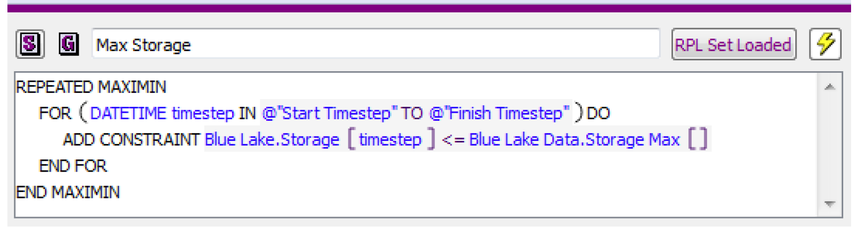
RiverWare will add the constraint shown in the goal to Optimization problem for every timestep (as a soft constraint), replacing the scalar slot Blue Lake Data.Storage Max with the actual value in the slot. Also, because this constraint references the Blue Lake Storage for every timestep, it will add the defining constraint for Blue Lake Storage, which is the mass balance constraint, for every timestep.

Notice that the mass balance constraint has also defined the variables for Inflow and Outflow at every timestep. Other variables could be included in the mass balance constraint as well, depending on the selected user methods on the reservoir (e.g. Hydrologic Inflow, Evaporation). RiverWare will also automatically add the upper and lower bound constraints for each of these three variables at each timestep based on the upper and lower bounds in the Slot Configuration for each; see Variable Bounds for details. If Inflow and Outflow are linked to slots on other objects, additional constraints will be added automatically which define the link relationship. In addition, a defining constraint will be added for Outflow setting it equal to the sum of Turbine Release and Spill, along with the upper and lower bound constraints for each of these new variables. So adding a single policy constraint can actually add numerous defining constraints for variables to the Optimization problem.
Physical Constraints
RiverWare automatically adds all relevant physical constraints to the Optimization problem. For example, the mass balance constraint for a reservoir is

This is the defining constraint for the Storage, Inflow and Outflow variables at time t. RiverWare determines which individual variables to include in Gains and Losses depending on the method selection on the reservoir. For example, Evaporation could be an additional loss variable in the mass balance constraint. For a reach, the defining physical constraints are determined by the selected routing method.
RiverWare only adds physical constraints as necessary based on the policy in the Optimization Goal Set. In this way it minimizes the size of the Optimization problem in order to achieve maximum computational efficiency. Physical constraints are always treated as hard constraints.
Variable Bounds
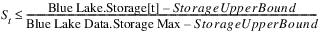
Upper and lower bounds are required for all decision variables. The bounds represent the absolute minimum and maximum for the slot (variable). The variable bounds remain constant and are automatically converted by RiverWare into hard constraints on the variable for every time step in the Optimization solution. They get used in defining constraint satisfaction for soft constraints. Soft constraint satisfaction is always scaled based on the difference between the constraint value (right-hand-side) and the previous bound, the RHS value from an earlier (higher priority) constraint with the same left-hand-side. If there is no earlier constraint with the same left-hand-side, then the previous bound is taken from the variable bounds. In other words, if a constraint in the Optimization goal set is the first constraint of its form, then the satisfaction of the constraint is calculated relative to the slot (variable) bound. For example, assume the following max storage goal is the first goal in the Optimization Goal Set (priority 1). See Figure 4.13.
Figure 4.13

The satisfaction St for the constraint on a single timestep would be as follows:

See Satisfaction Variables in Soft Constraints for details about how satisfaction variables in soft constraints are defined.
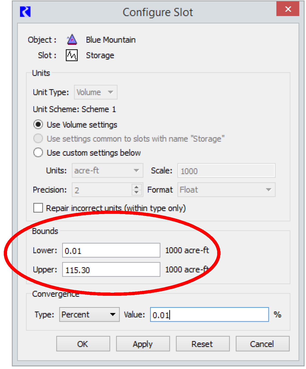
Often the variable bounds are based on the actual physical minimum and maximum. For example, the Storage Lower and Upper Bounds should be the smallest and largest Storage values in the Elevation Volume table. Turbine Release should be limited to zero as the Lower Bound and Turbine Capacity for the Upper Bound. In other cases, the absolute physical minimum or maximum may not be well-defined, such as maximum Inflow (or if economic variables are included in the model).
In these cases of variables without an obviously defined minimum or maximum, the slot bounds should not unnecessarily constrain the problem. These types of variables will typically be limited, either directly or indirectly, through the constraints in the Optimization Goal Set. It is also important, however, that the slot bounds not be set arbitrarily large or small (i.e. orders of magnitude different than the realistic limits) as this can result in numerical instability due to scaling issues in the optimization problem.
It is important that slot bounds not be confused with policy constraints, nor be used to apply policy constraints. For example, a hydropower plant might have a non-zero minimum generation requirement that it must meet, but the Power slot Lower Bound should still be zero. The minimum generation requirement would be set through a constraint in the Optimization Goal Set. The slot bounds become hard constraints in the optimization problem and essentially remain constant in the model, whereas policy constraint values (usually stored in custom slots) are typically incorporated as soft constraints and may change for different runs.
The slot bounds do not affect the Simulation solution. They are only applied in the Optimization solution. The Simulation solution is limited only by the physical characteristics described in table slots such as the Elevation Volume Table and Plant Power Table.
The variable bounds are displayed on the Configure Slot dialog. From the slot dialog select View, then Configure.
See Bounds on Variables for details about setting slot bounds in a model.
User-defined Variables
In addition to the set of standard variables that are automatically included in the Optimization problem, it is also possible to add customized user-defined variables. User-defined variables correspond to custom slots that the user adds to the model. The user must define the variables in a constraint that they add to the Goal Set. Then they can use the variable in a later policy constraint or objective.
There are five steps for implementing a user defined variable.
1. Add a series slot to an object in the model specifying appropriate units.
2. Specify that the slot is a user-defined variable.
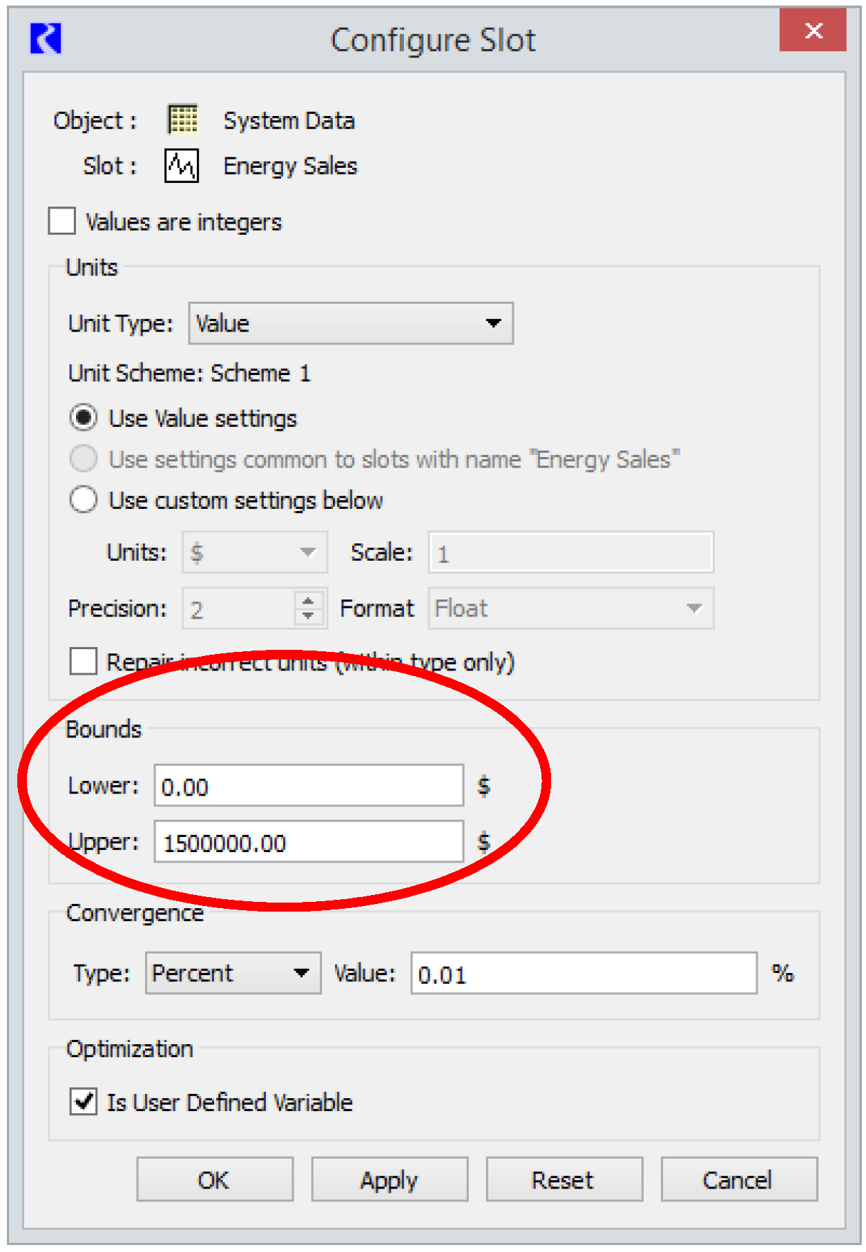
From the slot dialog select View, then Configure. In the resulting Configure Slot dialog, select the Is User Defined Variable check box, near the bottom of the dialog.
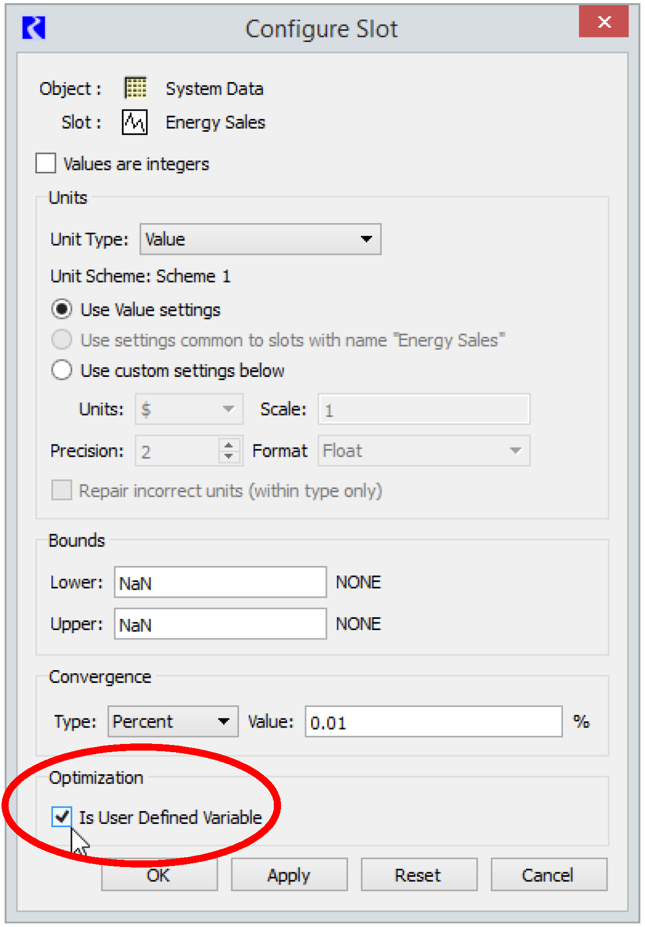
3. Set appropriate Lower and Upper Bounds for the variable in the Configure Slot dialog. See Variable Bounds for details about variable bounds.
4. Define the variable in a constraint in the Goal Set.
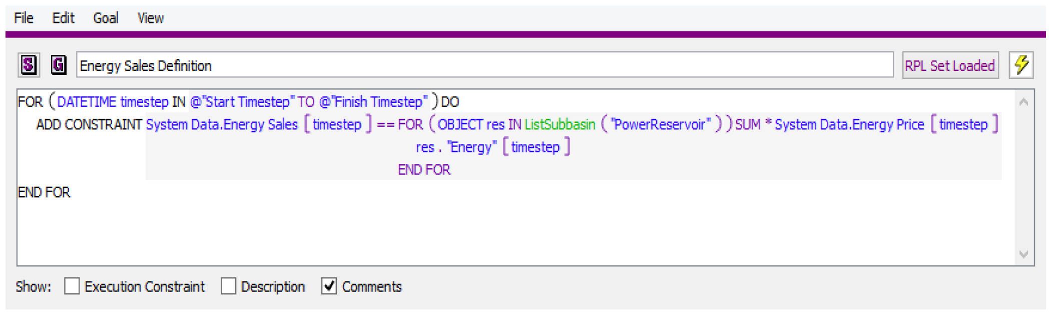
Figure 4.14 is an example that defines the variable Energy Sales at each time step as the total energy generation from all power reservoirs multiplied by the Energy Price. (This assumes that Energy Price is an input.) Variables are typically defined using hard constraints.
Figure 4.14
5. Use the variable in a policy constraint or objective.
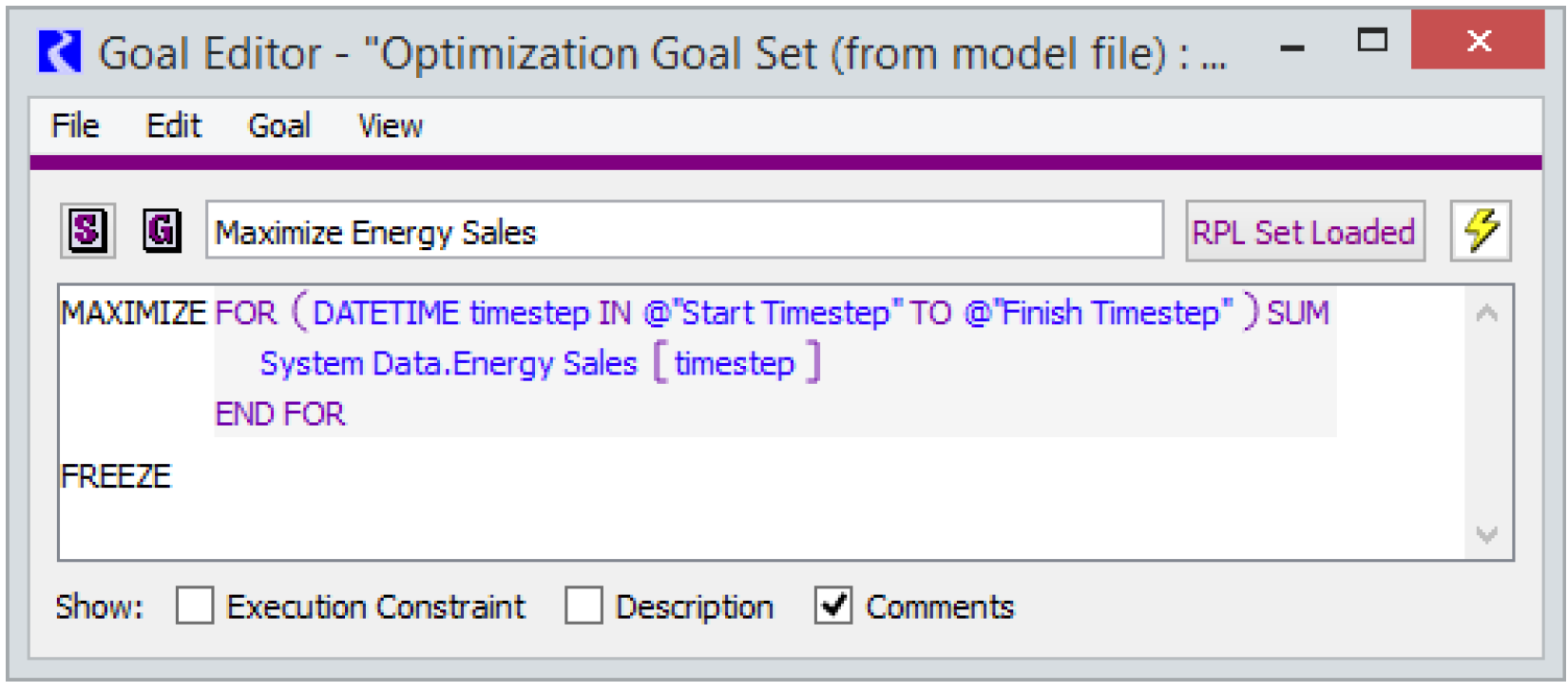
Figure 4.15 maximizes the sum over the entire run of the Energy Sales variable defined in the previous step.
Figure 4.15
User-defined variables provide much flexibility in extending the existing RiverWare methods for Optimization. The one restriction on user-defined variables is that, as with all Optimization constraints, the defining constraints must be linear expressions of other constraints.
Revised: 08/04/2020